SQL DS Interview
Sample Database: Awesome Chocolates
erDiagram
    GEO {
        varchar GeoID PK
        text Geo
        text Region
    }

    PEOPLE {
        varchar SPID PK
        text Salesperson
        text Team
        text Location
    }

    PRODUCTS {
        varchar PID PK
        text Product
        text Category
        text Size
        double Cost_per_box
    }

    SALES {
        text SPID
        text GeoID
        text PID
        datetime SaleDate
        int Amount
        int Customers
        int Boxes
    }

    PEOPLE ||--o{ SALES : makes
    GEO ||--o{ SALES : occurs_in
    PRODUCTS ||--o{ SALES : includes
Getting Started with SQL
Setting Up Your Environment
Tool Used: MySQL Workbench / BeeKeeper Studio
Database: Awesome Chocolates (must be downloaded and loaded)
Creating Your First Query
- Click the Plus SQL button in the corner to open the query editor
- View output results directly in the workbench grid
- Execute queries using Ctrl + Enter or the Run command
flowchart LR
    subgraph Query Execution Workflow
        A[Open Query Editor] --> B[Write SQL Query]
        B --> C[Execute Query]
        C --> D{Success?}
        D -->|Yes| E[View Results in Grid]
        D -->|No| F[Debug & Fix Errors]
        F --> B
    end
    style A fill:#1a1a2e,stroke:#4a9eff,color:#fff
    style B fill:#1a1a2e,stroke:#4a9eff,color:#fff
    style C fill:#1a1a2e,stroke:#4a9eff,color:#fff
    style D fill:#16213e,stroke:#f39c12,color:#fff
    style E fill:#0d3b0d,stroke:#2ecc71,color:#fff
style F fill:#3b0d0d,stroke:#e74c3c,color:#fffNote: Shortcuts differ depending on your system and SQL management tool:
- MySQL Workbench: Ctrl + Enter
- SQL Server Management Studio (SSMS): Different shortcut
- Oracle: Different shortcut
Understanding the Database Structure
Whenever you are getting started, take some minutes to know your db, it will help you build better sql queries !!!
Available Tables in Awesome Chocolates Database
The database contains four main tables:
- Geography table
- People table
- Products table
- Sales table
Exploring Table Contents
Before writing queries, understand your data structure.
View all tables in database:
| Tables_in_awesome chocolates |
|---|
| geo |
| people |
| products |
| sales |
...
View table structure and columns:
| Field | Type | Null | Key | Default | Extra |
|---|---|---|---|---|---|
| SPID | text | YES | null | ||
| GeoID | text | YES | null | ||
| PID | text | YES | null | ||
| SaleDate | datetime | YES | null | ||
| Amount | int | YES | null |
...
Actual mysql console response :
mysql> desc sales;
+-----------+----------+------+-----+---------+-------+
| Field     | Type     | Null | Key | Default | Extra |
+-----------+----------+------+-----+---------+-------+
| SPID      | text     | YES  |     | NULL    |       |
| GeoID     | text     | YES  |     | NULL    |       |
| PID       | text     | YES  |     | NULL    |       |
| SaleDate  | datetime | YES  |     | NULL    |       |
| Amount    | int      | YES  |     | NULL    |       |
| Customers | int      | YES  |     | NULL    |       |
| Boxes     | int      | YES  |     | NULL    |       |
+-----------+----------+------+-----+---------+-------+
7 rows in set (0.01 sec)

mysql>
What this returns:
- Column names
- Data types
- Additional information about each column
Important Concept
Critical Rule: When writing SQL queries, you must be familiar with underlying tables and their relationships. Without this knowledge, writing SQL becomes extremely difficult.
Output Display
Query Limit: MySQL Workbench displays a maximum of 1000 rows at a time, even if the table contains more data.
Example: Sales table contains ~7000 rows, but only 1000 display in the workbench
When to Adjust Limits:
- When building queries: You only need to verify it works correctly
- When exporting data: You may need to remove or increase the limit to see all data
- When using data elsewhere: Export to Power BI or other systems
Part 1: SELECT Statements and Basic Queries
SELECT All Columns
Query:
| SPID | GeoID | PID | SaleDate | Amount | Customers | Boxes |
|---|---|---|---|---|---|---|
| SP01 | G4 | P04 | 2021-01-01 00:00:00 | 8414 | 276 | 495 |
| SP02 | G3 | P14 | 2021-01-01 00:00:00 | 532 | 317 | 54 |
| SP12 | G2 | P08 | 2021-01-01 00:00:00 | 5376 | 178 | 269 |
| SP01 | G4 | P15 | 2021-01-01 00:00:00 | 259 | 32 | 22 |
| SP19 | G2 | P18 | 2021-01-01 00:00:00 | 5530 | 4 | 179 |
...
Explanation:
SELECT *means select everything (all columns)FROM salesspecifies the table name- Displays all rows and all columns from the sales table
Output: Complete sales table with all data visible in grid format
SELECT Specific Columns
Query:
| SaleDate | Amount | Customers |
|---|---|---|
| 2021-01-01 00:00:00 | 8414 | 276 |
| 2021-01-01 00:00:00 | 532 | 317 |
| 2021-01-01 00:00:00 | 5376 | 178 |
| 2021-01-01 00:00:00 | 259 | 32 |
| 2021-01-01 00:00:00 | 5530 | 4 |
...
Explanation:
- Specify only the columns you want to see
- Columns are separated by commas
- Result shows only these three columns for all rows
Auto-Suggest Feature: Type the table name first, then add columns. This enables auto-suggest to help prevent spelling mistakes.
Better Practice:
Then come back and add columns between SELECT and FROM.
Reordering Columns
Query:
| Amount | Customers | GeoID |
|---|---|---|
| 8414 | 276 | G4 |
| 532 | 317 | G3 |
| 5376 | 178 | G2 |
| 259 | 32 | G4 |
| 5530 | 4 | G2 |
...
Explanation:
- Columns do not have to appear in their original database order
- They display in the order you specify in the SELECT statement
- Results are rearranged automatically based on your specification
Adding Calculations to Queries
Calculate Amount Per Box:
| SaleDate | Amount | Boxes | Amount/Boxes |
|---|---|---|---|
| 2021-01-01 00:00:00 | 8414 | 495 | 16.9980 |
| 2021-01-01 00:00:00 | 532 | 54 | 9.8519 |
| 2021-01-01 00:00:00 | 5376 | 269 | 19.9851 |
| 2021-01-01 00:00:00 | 259 | 22 | 11.7727 |
| 2021-01-01 00:00:00 | 5530 | 179 | 30.8939 |
...
Explanation:
- You can perform arithmetic operations directly in SELECT statements
- Operations include addition (+), subtraction (-), multiplication (*), division (/)
- Results appear as an extra column in the output
- The calculated column name defaults to the operation itself
Creating Aliases for Calculated Columns
Problem: Column name amount / boxes is not user-friendly
Solution: Add Column Aliases Using AS:
| SaleDate | Amount | Boxes | amount_per_box |
|---|---|---|---|
| 2021-01-01 00:00:00 | 8414 | 495 | 16.9980 |
| 2021-01-01 00:00:00 | 532 | 54 | 9.8519 |
| 2021-01-01 00:00:00 | 5376 | 269 | 19.9851 |
| 2021-01-01 00:00:00 | 259 | 22 | 11.7727 |
| 2021-01-01 00:00:00 | 5530 | 179 | 30.8939 |
...
Alternative Without AS Keyword:
| SaleDate | Amount | Boxes | amount_per_box |
|---|---|---|---|
| 2021-01-01 00:00:00 | 8414 | 495 | 16.9980 |
| 2021-01-01 00:00:00 | 532 | 54 | 9.8519 |
| 2021-01-01 00:00:00 | 5376 | 269 | 19.9851 |
| 2021-01-01 00:00:00 | 259 | 22 | 11.7727 |
| 2021-01-01 00:00:00 | 5530 | 179 | 30.8939 |
| SaleDate | Amount | Boxes | amount per box |
|---|---|---|---|
| 2021-01-01 00:00:00 | 8414 | 495 | 16.9980 |
| 2021-01-01 00:00:00 | 532 | 54 | 9.8519 |
| 2021-01-01 00:00:00 | 5376 | 269 | 19.9851 |
| 2021-01-01 00:00:00 | 259 | 22 | 11.7727 |
| 2021-01-01 00:00:00 | 5530 | 179 | 30.8939 |
Note: Both methods produce identical results. The AS keyword creates a synonym for the column.
Key Takeaway on Aliases
The alias makes your output more readable and professional. Many times you want to give calculated columns proper names for clarity.
Part 2: WHERE Clauses - Filtering Data
Understanding WHERE Clauses
Definition: The WHERE clause allows you to impose conditions on your query results.
Concept: WHERE clause in SQL is like filtering in Excel. Set filter criteria to show only specific data.
Importance: WHERE clauses are one of the most important aspects of SQL for data analysis.
flowchart LR
subgraph WHERE Clause Flow
A[All Rows] --> B{Evaluate Condition}
B -->|TRUE| C[Include Row]
B -->|FALSE| D[Exclude Row]
C --> E[Result Set]
D --> F[Discarded]
end
style A fill:#1a1a2e,stroke:#4a9eff,color:#fff
style B fill:#16213e,stroke:#f39c12,color:#fff
style C fill:#0d3b0d,stroke:#2ecc71,color:#fff
style D fill:#3b0d0d,stroke:#e74c3c,color:#fff
style E fill:#1a1a2e,stroke:#4a9eff,color:#fff
style F fill:#2d2d2d,stroke:#666,color:#999Basic WHERE Clause with Greater Than
Query:
| SPID | GeoID | PID | SaleDate | Amount | Customers | Boxes |
|---|---|---|---|---|---|---|
| SP06 | G4 | P01 | 2021-01-01 00:00:00 | 12894 | 115 | 478 |
| SP10 | G1 | P06 | 2021-01-01 00:00:00 | 15596 | 32 | 975 |
| SP25 | G6 | P05 | 2021-01-01 00:00:00 | 14273 | 335 | 752 |
| SP18 | G2 | P21 | 2021-01-04 00:00:00 | 19229 | 64 | 1013 |
| SP23 | G1 | P16 | 2021-01-05 00:00:00 | 17248 | 163 | 664 |
...
Explanation:
WHEREspecifies the filter conditionamount > 10000means only rows where amount is greater than 10,000- All rows where amount is NOT greater than 10,000 are excluded
- Only qualifying rows display in results
Comparison Operators:
>Greater than<Less than=Equal to>=Greater than or equal to<=Less than or equal to!=or<>Not equal to
Combining WHERE with ORDER BY
Query:
| SPID | GeoID | PID | SaleDate | Amount | Customers | Boxes |
|---|---|---|---|---|---|---|
| SP02 | G1 | P07 | 2021-09-17 00:00:00 | 10010 | 257 | 358 |
| SP01 | G2 | P17 | 2021-08-30 00:00:00 | 10017 | 163 | 835 |
| SP21 | G3 | P22 | 2021-11-18 00:00:00 | 10017 | 111 | 418 |
| SP18 | G5 | P18 | 2021-10-27 00:00:00 | 10017 | 77 | 1113 |
| SP23 | G5 | P03 | 2021-05-06 00:00:00 | 10024 | 32 | 627 |
...
Explanation:
- Filters results to show only amounts greater than 10,000
- Orders results by amount in ascending order (lowest to highest)
- Results start at 10,000+ and increase gradually
Ascending Order (Default):
| SPID | GeoID | PID | SaleDate | Amount | Customers | Boxes |
|---|---|---|---|---|---|---|
| SP02 | G1 | P07 | 2021-09-17 00:00:00 | 10010 | 257 | 358 |
| SP01 | G2 | P17 | 2021-08-30 00:00:00 | 10017 | 163 | 835 |
| SP21 | G3 | P22 | 2021-11-18 00:00:00 | 10017 | 111 | 418 |
| SP18 | G5 | P18 | 2021-10-27 00:00:00 | 10017 | 77 | 1113 |
| SP23 | G5 | P03 | 2021-05-06 00:00:00 | 10024 | 32 | 627 |
...
Descending Order (Highest to Lowest):
| SPID | GeoID | PID | SaleDate | Amount | Customers | Boxes |
|---|---|---|---|---|---|---|
| SP23 | G4 | P03 | 2021-02-12 00:00:00 | 27146 | 329 | 1939 |
| SP18 | G5 | P10 | 2021-04-22 00:00:00 | 25207 | 22 | 1483 |
| SP03 | G5 | P22 | 2021-06-02 00:00:00 | 24633 | 39 | 986 |
| SP18 | G1 | P11 | 2021-10-21 00:00:00 | 24451 | 472 | 1112 |
| SP18 | G2 | P16 | 2021-03-30 00:00:00 | 24367 | 272 | 3481 |
...
Multiple Sort Criteria
Query:
| SPID | GeoID | PID | SaleDate | Amount | Customers | Boxes |
|---|---|---|---|---|---|---|
| SP14 | G1 | P01 | 2022-02-25 00:00:00 | 22897 | 43 | 1347 |
| SP21 | G1 | P01 | 2022-01-07 00:00:00 | 18130 | 24 | 1008 |
| SP11 | G1 | P01 | 2021-01-27 00:00:00 | 17402 | 43 | 697 |
| SP08 | G1 | P01 | 2021-09-13 00:00:00 | 16681 | 274 | 596 |
| SP08 | G1 | P01 | 2022-01-10 00:00:00 | 16121 | 55 | 896 |
...
Explanation:
- Filters to show only GeoID 'g1' records
- First sorts by product ID (pid)
- Within each product ID, sorts by amount in descending order
- You can specify multiple ORDER BY columns separated by commas
Result Structure:
- All p01 items grouped together, sorted by amount (highest first)
- Then p02 items grouped together, sorted by amount
- Then p03, p04, etc.
WHERE Clause with AND Operator
Scenario: Find all sales with amount > 10,000 in the year 2022
Query Method 1 - Using Date Comparison:
SELECT * FROM sales
WHERE amount > 10000
AND saledate >= '2022-01-01';
-- use quote in dates `2022-01-01' : correct, 2022-01-01 : incorrect
| SPID | GeoID | PID | SaleDate | Amount | Customers | Boxes |
|---|---|---|---|---|---|---|
| SP15 | G3 | P11 | 2022-01-05 00:00:00 | 14553 | 152 | 910 |
| SP16 | G3 | P22 | 2022-01-28 00:00:00 | 10255 | 53 | 733 |
| SP04 | G4 | P05 | 2022-01-28 00:00:00 | 16800 | 92 | 800 |
| SP05 | G1 | P02 | 2022-01-21 00:00:00 | 16121 | 487 | 621 |
| SP21 | G2 | P22 | 2022-01-11 00:00:00 | 12481 | 177 | 1041 |
...
Explanation:
- Filters to amount greater than 10,000
- AND date is within 2022 or later
- Both conditions must be true for rows to display
MySQL Date Format: YYYY-MM-DD
Date Example: 2022-01-01 represents January 1st, 2022
Using YEAR Function with WHERE
Query Method 2 - Using YEAR Function:
SELECT saledate, amount
FROM sales
WHERE amount > 10000
AND YEAR(saledate) = 2022
ORDER BY amount DESC;
| saledate | amount |
|---|---|
| 2022-02-16 00:00:00 | 23912 |
| 2022-03-15 00:00:00 | 23184 |
| 2022-02-25 00:00:00 | 22897 |
| 2022-03-01 00:00:00 | 22603 |
| 2022-02-25 00:00:00 | 22155 |
...
Explanation:
YEAR()is a built-in SQL function that extracts the year from a date- Works similar to YEAR function in Excel
- Returns a number, so no quotes needed around 2022
- More flexible than date comparison method
Advantage: Cleaner and more maintainable than parsing dates manually
WHERE Clause with BETWEEN
Scenario: Find all sales with boxes between 0 and 50
Query Method 1 - Using AND:
| SPID | GeoID | PID | SaleDate | Amount | Customers | Boxes |
|---|---|---|---|---|---|---|
| SP01 | G4 | P15 | 2021-01-01 00:00:00 | 259 | 32 | 22 |
| SP14 | G5 | P16 | 2021-01-01 00:00:00 | 1036 | 370 | 37 |
| SP12 | G6 | P09 | 2021-01-04 00:00:00 | 147 | 9 | 11 |
| SP04 | G1 | P20 | 2021-01-06 00:00:00 | 644 | 116 | 34 |
| SP10 | G2 | P01 | 2021-01-08 00:00:00 | 420 | 196 | 14 |
...
Query Method 2 - Using BETWEEN(it includes limits):
| SPID | GeoID | PID | SaleDate | Amount | Customers | Boxes |
|---|---|---|---|---|---|---|
| SP01 | G4 | P15 | 2021-01-01 00:00:00 | 259 | 32 | 22 |
| SP14 | G5 | P16 | 2021-01-01 00:00:00 | 1036 | 370 | 37 |
| SP12 | G6 | P09 | 2021-01-04 00:00:00 | 147 | 9 | 11 |
| SP04 | G1 | P20 | 2021-01-06 00:00:00 | 644 | 116 | 34 |
| SP10 | G2 | P01 | 2021-01-08 00:00:00 | 420 | 196 | 14 |
...
Explanation:
- BETWEEN is inclusive on both ends
- Range includes 0 and 50
- Both methods produce the same results
- BETWEEN is more concise and readable
Note: Both methods are valid. Use whichever is more comfortable for you.
Weekday Function Example
Scenario: Find all sales that occurred on Fridays
Query:
SELECT
saledate,
amount,
boxes,
WEEKDAY(saledate) AS day_of_week
FROM sales
WHERE WEEKDAY(saledate) = 4;
| SaleDate | Amount | Boxes | day_of_week |
|---|---|---|---|
| 2021-01-01 00:00:00 | 8414 | 495 | 4 |
| 2021-01-01 00:00:00 | 532 | 54 | 4 |
| 2021-01-01 00:00:00 | 5376 | 269 | 4 |
| 2021-01-01 00:00:00 | 259 | 22 | 4 |
| 2021-01-01 00:00:00 | 5530 | 179 | 4 |
Explanation:
WEEKDAY()is a built-in function that returns day of week as a number- Weekday numbering: 0=Monday, 1=Tuesday, 2=Wednesday, 3=Thursday, 4=Friday, 5=Saturday, 6=Sunday
- Friday = 4, so the condition is
WEEKDAY(SaleDate) = 4 - Can also create alias
AS day_of_weekfor clarity
Important Note: When using a calculated column in WHERE clause, you cannot reference the alias. You must repeat the calculation:
Part 3: Logical Operators - AND, OR, NOT
The OR Operator
Scenario: Find all people in either "Delish" or "Juices" team
Query Method 1 - Using Multiple OR Conditions:
| Salesperson | SPID | Team | Location |
|---|---|---|---|
| Wilone O'Kielt | SP04 | Delish | Hyderabad |
| Gigi Bohling | SP05 | Delish | Hyderabad |
| Curtice Advani | SP06 | Delish | Hyderabad |
| Kaine Padly | SP07 | Delish | Hyderabad |
| Andria Kimpton | SP09 | Jucies | Hyderabad |
...
Explanation:
- Shows results where team equals 'Delish' OR team equals 'Juices'
- Either condition being true includes the row
- Person cannot be in both teams, so OR is appropriate
Limitation: If you need many possible values, OR conditions become repetitive and difficult to maintain
The IN Operator
Query Method 2 - Using IN (Cleaner Approach):
| Salesperson | SPID | Team | Location |
|---|---|---|---|
| Wilone O'Kielt | SP04 | Delish | Hyderabad |
| Gigi Bohling | SP05 | Delish | Hyderabad |
| Curtice Advani | SP06 | Delish | Hyderabad |
| Kaine Padly | SP07 | Delish | Hyderabad |
| Andria Kimpton | SP09 | Jucies | Hyderabad |
...
Explanation:
INis shorthand for multiple OR conditions- Specify multiple values in parentheses, separated by commas
- All text values must be in single quotes
- More flexible when you have many possible values
- More readable and maintainable
Advantage over OR: When you need 5, 7, or 10+ possible values, IN is much cleaner than chaining multiple OR conditions.
The LIKE Operator - Pattern Matching
Scenario: Find all people whose name begins with 'B'
Query:
| Salesperson | SPID | Team | Location |
|---|---|---|---|
| Barr Faughny | SP01 | Yummies | Hyderabad |
| Brien Boise | SP10 | Jucies | Wellington |
| Beverie Moffet | SP19 | Jucies | Seattle |
| Benny Karolovsky | SP32 | Jucies | Paris |
...
Explanation:
LIKEoperator performs pattern matchingB%means: starts with 'B', followed by anything (%)%is a wildcard meaning "any character, zero or more times"- Names starting with B: Boris, Bonnie, etc.
Pattern Matching Examples:
Find names starting with B:
| Salesperson | SPID | Team | Location |
|---|---|---|---|
| Barr Faughny | SP01 | Yummies | Hyderabad |
| Brien Boise | SP10 | Jucies | Wellington |
| Beverie Moffet | SP19 | Jucies | Seattle |
| Benny Karolovsky | SP32 | Jucies | Paris |
Find names containing B anywhere:
| Salesperson | SPID | Team | Location |
|---|---|---|---|
| Barr Faughny | SP01 | Yummies | Hyderabad |
| Gigi Bohling | SP05 | Delish | Hyderabad |
| Ches Bonnell | SP08 | Hyderabad | |
| Brien Boise | SP10 | Jucies | Wellington |
| Marney O'Breen | SP16 | Jucies | Wellington |
...
Find names ending with l:
| Salesperson | SPID | Team | Location |
|---|---|---|---|
| Ches Bonnell | SP08 | Hyderabad | |
| Oby Sorrel | SP20 | Jucies | Seattle |
| Van Tuxwell | SP23 | Yummies | Seattle |
...
Find names with B as second character:
| Salesperson | SPID | Team | Location |
|---|---|---|---|
| Oby Sorrel | SP20 | Jucies | Seattle |
| Ebonee Roxburgh | SP28 | Paris |
...
(Where _ means exactly one character)
The NOT Operator
Scenario: Find sales where the team is NOT equal to a specific value
Query:
select * from products
where Category != 'Bars';
-- OR --
select * from products
where Category <> 'Bars';
-- OR --
select * from products
where not (Category = 'Bars');
| PID | Product | Category | Size | Cost_per_box |
|---|---|---|---|---|
| P02 | 50% Dark Bites | Bites | LARGE | 2.57 |
| P06 | Eclairs | Bites | LARGE | 2.24 |
| P07 | Drinking Coco | Other | LARGE | 1.62 |
| P10 | Spicy Special Slims | Bites | LARGE | 5.79 |
| P11 | After Nines | Bites | LARGE | 4.43 |
| P14 | White Choc | Other | SMALL | 0.16 |
...
Explanation:
!=and<>both mean "not equal to"NOToperator reverses a condition- All three queries produce identical results
Part 4: Conditional Logic with CASE
Understanding CASE Statements
Purpose: Create categorizations or conditional logic within SELECT statements
Scenario: Categorize sales amounts into different tiers:
- Under $1,000: "Under 1K"
- $1,000 to $5,000: "Under 5K"
- $5,000 to $10,000: "Under 10K"
- Over $10,000: "10K or More"
flowchart TD
subgraph CASE Statement Evaluation
A[Input Value] --> B{Amount < 1000?}
B -->|Yes| C["Under 1K"]
B -->|No| D{Amount < 5000?}
D -->|Yes| E["Under 5K"]
D -->|No| F{Amount < 10000?}
F -->|Yes| G["Under 10K"]
F -->|No| H["10K or More"]
end
style A fill:#1a1a2e,stroke:#4a9eff,color:#fff
style B fill:#16213e,stroke:#f39c12,color:#fff
style C fill:#0d3b0d,stroke:#2ecc71,color:#fff
style D fill:#16213e,stroke:#f39c12,color:#fff
style E fill:#0d3b0d,stroke:#2ecc71,color:#fff
style F fill:#16213e,stroke:#f39c12,color:#fff
style G fill:#0d3b0d,stroke:#2ecc71,color:#fff
style H fill:#0d3b0d,stroke:#2ecc71,color:#fffCASE Statement Structure
Query:
select SaleDate,Amount ,case when Amount < 1000 then 'Under 1K' when Amount < 5000 then 'Under 2K' when Amount < 10000 then 'Under 10K' else '10K or More' end as amount_category from sales ;
| SaleDate | Amount | amount_category |
|---|---|---|
| 2021-01-01 00:00:00 | 8414 | Under 10K |
| 2021-01-01 00:00:00 | 532 | Under 1K |
| 2021-01-01 00:00:00 | 5376 | Under 10K |
| 2021-01-01 00:00:00 | 259 | Under 1K |
| 2021-01-01 00:00:00 | 5530 | Under 10K |
...
Explanation:
CASEbegins the conditional logicWHEN condition THEN resultchecks each condition sequentially- Conditions are evaluated in order from top to bottom
- First matching condition returns its result
ELSEprovides default value if no conditions matchENDterminates the CASE statement- Assign alias
AS amount_categoryto name the result column
CASE with Multiple Conditions
You can use multiple WHEN statements and combine conditions as needed.
Query Structure Best Practices:
For clarity in longer queries, break CASE statements into multiple lines:
SELECT
saledate,
amount
,CASE
WHEN amount < 1000 THEN 'Under 1K'
WHEN amount < 5000 THEN 'Under 5K'
WHEN amount < 10000 THEN 'Under 10K'
ELSE '10K or More'
END AS amount_category
FROM sales;
| SaleDate | Amount | amount_category |
|---|---|---|
| 2021-01-01 00:00:00 | 8414 | Under 10K |
| 2021-01-01 00:00:00 | 532 | Under 1K |
| 2021-01-01 00:00:00 | 5376 | Under 10K |
| 2021-01-01 00:00:00 | 259 | Under 1K |
| 2021-01-01 00:00:00 | 5530 | Under 10K |
...
Use Cases for CASE
- Create numeric categorizations
- Create text-based categorizations
- Use in WHERE clause to filter on categorizations
- Map values for reporting and analysis
- Create custom display values
Part 5: JOINs - Combining Multiple Tables
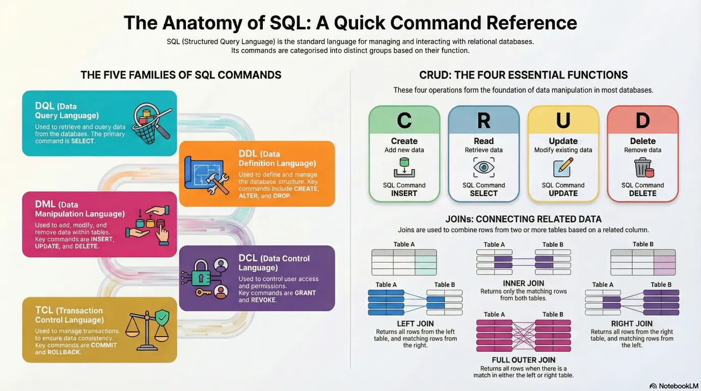
Understanding JOINs
Definition: JOINs combine data from multiple tables based on related columns.
Concept: Similar to VLOOKUP in Excel, but SQL uses more optimized methods.
Critical Prerequisite: Understand how tables are linked through foreign keys before attempting JOINs.
flowchart LR
subgraph "JOIN Types"
direction TB
subgraph INNER["INNER JOIN"]
I1[Table A] --- IM((Matching)) --- I2[Table B]
end
subgraph LEFT["LEFT JOIN"]
L1[All A] --- LM((Matching)) --- L2[Matched B]
end
subgraph RIGHT["RIGHT JOIN"]
R1[Matched A] --- RM((Matching)) --- R2[All B]
end
end
style I1 fill:#1a1a2e,stroke:#4a9eff,color:#fff
style I2 fill:#1a1a2e,stroke:#4a9eff,color:#fff
style IM fill:#16213e,stroke:#2ecc71,color:#fff
style L1 fill:#0d3b0d,stroke:#2ecc71,color:#fff
style L2 fill:#1a1a2e,stroke:#4a9eff,color:#fff
style LM fill:#16213e,stroke:#f39c12,color:#fff
style R1 fill:#1a1a2e,stroke:#4a9eff,color:#fff
style R2 fill:#0d3b0d,stroke:#2ecc71,color:#fff
style RM fill:#16213e,stroke:#f39c12,color:#fff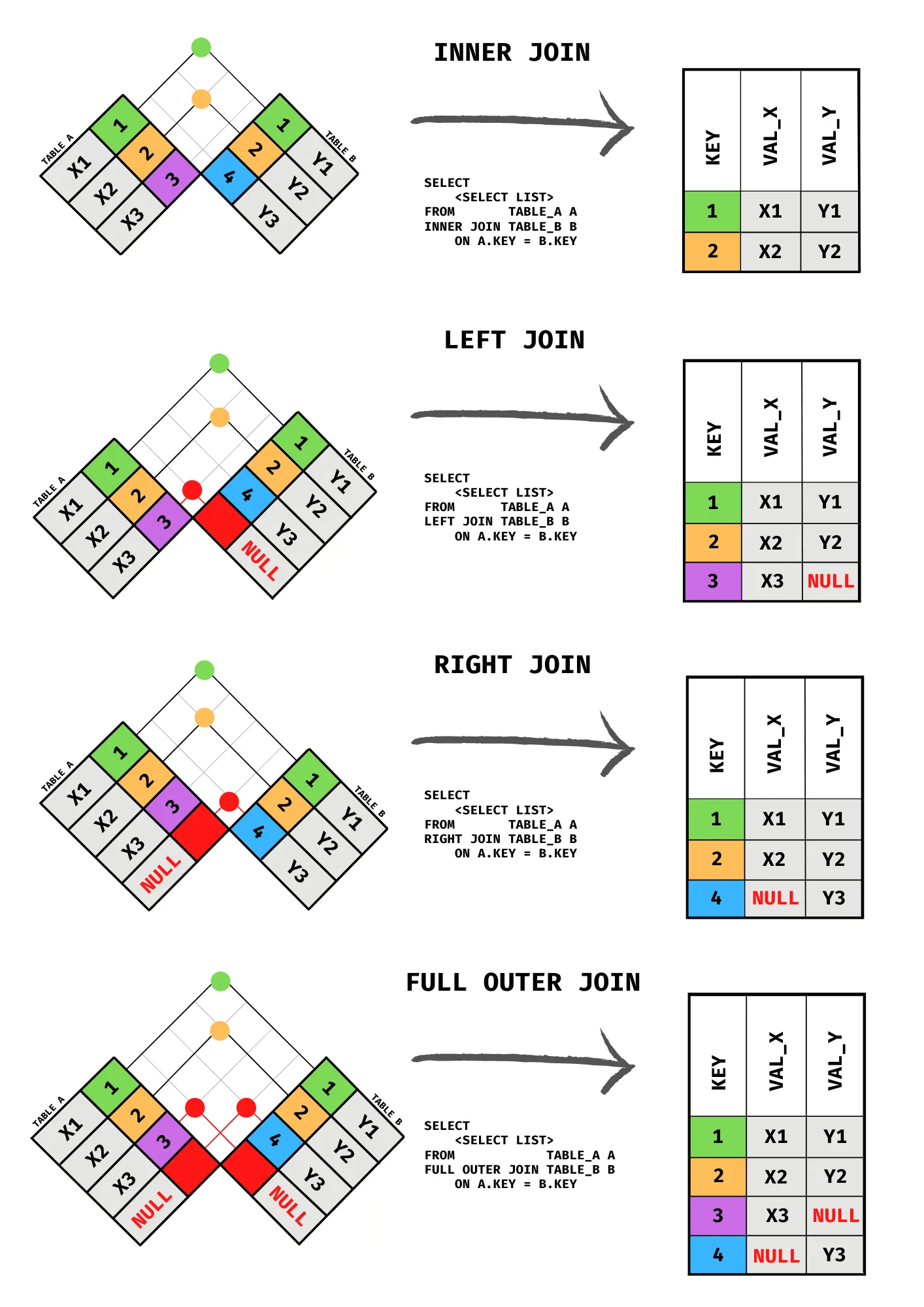
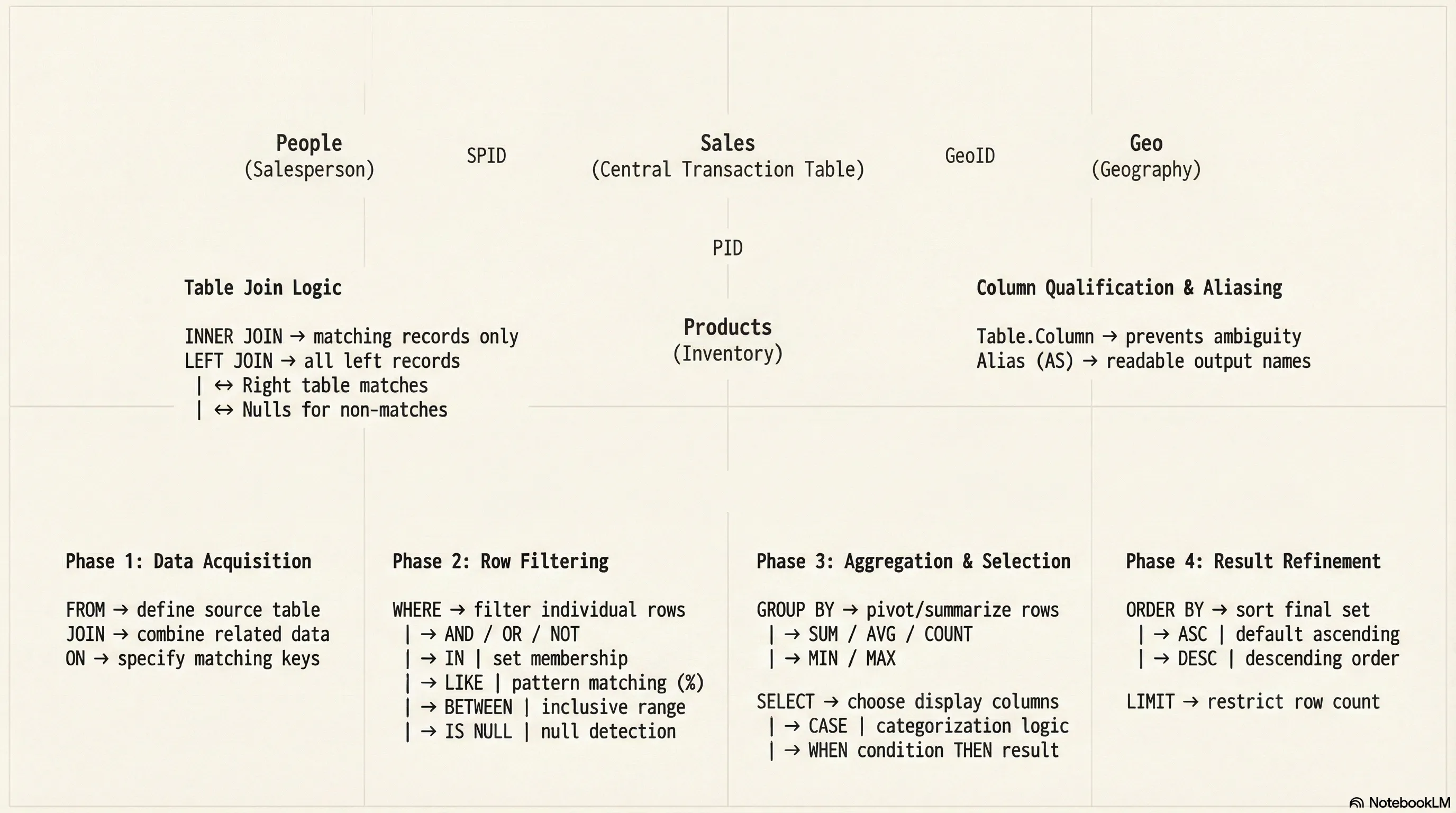
Database Relationships in Awesome Chocolates
Table Relationships:
- Sales table contains:
SPID(links to People table) - Sales table contains:
pid(links to Products table) - Sales table contains:
GeoID(links to Geography table)
Principle: IDs that appear in multiple tables represent the same entity and can be used to JOIN tables.
Basic JOIN Example
Scenario: Show sales data with the person's name instead of just ID
Without JOIN - Problem:
| SPID | GeoID | PID | SaleDate | Amount | Customers | Boxes |
|---|---|---|---|---|---|---|
| SP01 | G4 | P04 | 2021-01-01 00:00:00 | 8414 | 276 | 495 |
| SP02 | G3 | P14 | 2021-01-01 00:00:00 | 532 | 317 | 54 |
| SP12 | G2 | P08 | 2021-01-01 00:00:00 | 5376 | 178 | 269 |
| SP01 | G4 | P15 | 2021-01-01 00:00:00 | 259 | 32 | 22 |
| SP19 | G2 | P18 | 2021-01-01 00:00:00 | 5530 | 4 | 179 |
...
With JOIN - Solution:
| SaleDate | Amount | Salesperson |
|---|---|---|
| 2021-01-01 00:00:00 | 8414 | Barr Faughny |
| 2021-01-01 00:00:00 | 532 | Dennison Crosswaite |
| 2021-01-01 00:00:00 | 5376 | Karlen McCaffrey |
| 2021-01-01 00:00:00 | 259 | Barr Faughny |
| 2021-01-01 00:00:00 | 5530 | Beverie Moffet |
...
select
s.SaleDate,
s.Amount,
p.Salesperson,
s.SPID,
p.SPID
from sales s
join people p on p.SPID = s.SPID
;
| SaleDate | Amount | Salesperson | SPID |
|---|---|---|---|
| 2021-01-01 00:00:00 | 8414 | Barr Faughny | SP01 |
| 2021-01-01 00:00:00 | 532 | Dennison Crosswaite | SP02 |
| 2021-01-01 00:00:00 | 5376 | Karlen McCaffrey | SP12 |
| 2021-01-01 00:00:00 | 259 | Barr Faughny | SP01 |
| 2021-01-01 00:00:00 | 5530 | Beverie Moffet | SP19 |
Explanation:
FROM sales sstarts with sales table, aliased as 's'JOIN people padds the people table, aliased as 'p'ON p.SPID = s.SPIDspecifies the join condition - matching IDss.andp.prefixes specify which table a column comes from- When IDs match, data from both tables appears on the same row
Table Aliases
Purpose: Shorten long table names and make queries more readable
Syntax:
Consistency Practice: Use consistent aliases within your query. Example:
sfor salespfor peopleprfor productsgfor geo
Column Qualification
Why Qualify Columns with Table Prefix?
When columns have the same name in multiple tables, prefix with table alias:
Best Practice: Even when not required, qualify columns for clarity.
LEFT JOIN vs JOIN
JOIN (INNER JOIN):
- Returns only rows where IDs match in BOTH tables
- If sales table has SPID that doesn't exist in people table, that row is excluded
LEFT JOIN:
- Returns ALL rows from the left table (first table after FROM)
- Includes matching rows from the right table
- If no match found, right table columns show as blank/NULL
- Used to preserve all data from the primary table
Visual Representation:
Sales table (LEFT) ----------- People table (RIGHT)
[Keep ALL from sales]
[If match in people → Include people data]
[If no match in people → Show blank for people columns]
When to Use LEFT JOIN: Most common in business situations because you want to preserve all sales data even if the person's record doesn't exist in the people table.
| SaleDate | Amount | Product |
|---|---|---|
| 2021-01-01 00:00:00 | 8414 | Raspberry Choco |
| 2021-01-01 00:00:00 | 532 | White Choc |
| 2021-01-01 00:00:00 | 5376 | 99% Dark & Pure |
| 2021-01-01 00:00:00 | 259 | Baker's Choco Chips |
| 2021-01-01 00:00:00 | 5530 | Manuka Honey Choco |
...
| SaleDate | Amount | Product |
|---|---|---|
| 2022-03-23 00:00:00 | 637 | Milk Bars |
| 2022-02-25 00:00:00 | 2730 | Milk Bars |
| 2022-02-24 00:00:00 | 9023 | Milk Bars |
| 2022-03-04 00:00:00 | 1155 | Milk Bars |
| 2022-03-30 00:00:00 | 1120 | Milk Bars |
...
JOIN with WHERE Clause
Scenario: Show sales under $500 for people in the "Delish" team
Query:
SELECT
s.SaleDate,
s.amount,
p.salesperson,
p.team
FROM sales s
JOIN people p ON p.SPID = s.SPID
WHERE s.amount < 500
AND p.team = 'Delish';
| SaleDate | Amount | Salesperson | Team |
|---|---|---|---|
| 2021-01-08 00:00:00 | 364 | Gigi Bohling | Delish |
| 2021-01-14 00:00:00 | 35 | Jan Morforth | Delish |
| 2021-01-15 00:00:00 | 308 | Curtice Advani | Delish |
| 2021-02-04 00:00:00 | 182 | Camilla Castle | Delish |
| 2021-02-04 00:00:00 | 392 | Jan Morforth | Delish |
...
Explanation:
- JOIN combines the tables
- WHERE clause filters results on joined data
- Can filter on any column from either table
for fun, see the empty stuff !!!
select
s.SaleDate,
s.Amount,
p.Salesperson,
p.Team
from sales s
join people p on p.SPID = s.SPID
where s.Amount< 500
;
| SaleDate | Amount | Salesperson | Team |
|---|---|---|---|
| 2021-01-01 00:00:00 | 259 | Barr Faughny | Yummies |
| 2021-01-04 00:00:00 | 147 | Karlen McCaffrey | Yummies |
| 2021-01-08 00:00:00 | 420 | Brien Boise | Jucies |
| 2021-01-08 00:00:00 | 364 | Gigi Bohling | Delish |
| 2021-01-08 00:00:00 | 357 | Ches Bonnell | |
| 2021-01-12 00:00:00 | 189 | Husein Augar | Yummies |
| 2021-01-12 00:00:00 | 490 | Barr Faughny | Yummies |
| 2021-01-14 00:00:00 | 35 | Jan Morforth | Delish |
| 2021-01-15 00:00:00 | 308 | Curtice Advani | Delish |
| 2021-01-18 00:00:00 | 238 | Brien Boise | Jucies |
| 2021-01-19 00:00:00 | 161 | Ches Bonnell | |
| 2021-01-20 00:00:00 | 343 | Brien Boise | Jucies |
| 2021-01-20 00:00:00 | 126 | Kelci Walkden | Yummies |
| 2021-01-21 00:00:00 | 280 | Ches Bonnell | |
| 2021-01-21 00:00:00 | 427 | Marney O'Breen | Jucies |
| 2021-01-22 00:00:00 | 168 | Oby Sorrel | Jucies |
| 2021-01-25 00:00:00 | 42 | Ches Bonnell | |
| 2021-01-25 00:00:00 | 343 | Mallorie Waber |
...
select
s.SaleDate,
s.Amount,
p.Salesperson,
p.Team
from sales s
join people p on p.SPID = s.SPID
where s.Amount< 500
and p.Team = ''
;
| SaleDate | Amount | Salesperson | Team |
|---|---|---|---|
| 2021-01-08 00:00:00 | 357 | Ches Bonnell | |
| 2021-01-19 00:00:00 | 161 | Ches Bonnell | |
| 2021-01-21 00:00:00 | 280 | Ches Bonnell | |
| 2021-01-25 00:00:00 | 42 | Ches Bonnell | |
| 2021-01-25 00:00:00 | 343 | Mallorie Waber |
...
Multiple JOINs
Scenario: Show sales with person name, product name, and team
Query:
SELECT
s.SaleDate,
s.amount,
p.salesperson,
pr.product,
p.team
FROM sales s
JOIN people p ON p.SPID = s.SPID
JOIN products pr ON pr.pid = s.pid;
| SaleDate | Amount | Salesperson | Product | Team |
|---|---|---|---|---|
| 2021-01-01 00:00:00 | 8414 | Barr Faughny | Raspberry Choco | Yummies |
| 2021-01-01 00:00:00 | 532 | Dennison Crosswaite | White Choc | Yummies |
| 2021-01-01 00:00:00 | 5376 | Karlen McCaffrey | 99% Dark & Pure | Yummies |
| 2021-01-01 00:00:00 | 259 | Barr Faughny | Baker's Choco Chips | Yummies |
| 2021-01-01 00:00:00 | 5530 | Beverie Moffet | Manuka Honey Choco | Jucies |
| 2021-01-01 00:00:00 | 2184 | Rafaelita Blaksland | 85% Dark Bars |
...
Explanation:
- Chain multiple JOINs by adding additional JOIN clauses
- Each JOIN specifies its own ON condition
- Data from all three tables appears in result
- Order of JOINs: START with FROM clause, then add each JOIN sequentially
JOIN with Null Handling
Problem: Some people records might not have a team assigned (blank or NULL)
Query:
SELECT
s.SaleDate,
s.amount,
p.salesperson,
p.team
FROM sales s
LEFT JOIN people p ON p.SPID = s.SPID
WHERE s.amount < 500
AND p.team IS NULL; -- p.team = ''
| SaleDate | Amount | Salesperson | Team |
|---|---|---|---|
| 2021-01-08 00:00:00 | 357 | Ches Bonnell | |
| 2021-01-19 00:00:00 | 161 | Ches Bonnell | |
| 2021-01-21 00:00:00 | 280 | Ches Bonnell | |
| 2021-01-25 00:00:00 | 42 | Ches Bonnell | |
| 2021-01-25 00:00:00 | 343 | Mallorie Waber |
...
Explanation:
IS NULLchecks for NULL values (true null, not blank spaces)IS NOT NULLchecks for non-null values
Database Nuance: Null vs Blank
- NULL: Truly no value assigned (appears as "NULL" in results)
- Blank: Empty string or spaces (appears as empty in results)
Different filtering required for each:
- NULL:
WHERE column IS NULL - Blank:
WHERE column = ''
Three-Table JOIN Example
Complete Query with Multiple Filters:
SELECT
s.SaleDate,
s.amount,
p.salesperson,
pr.product,
g.geo
FROM sales s
JOIN people p ON p.SPID = s.SPID
JOIN products pr ON pr.pid = s.pid
JOIN geo g ON g.GeoID = s.GeoID
WHERE s.amount < 500
AND p.team = ''
AND g.geo IN ('New Zealand', 'India')
ORDER BY s.SaleDate;
| SaleDate | Amount | Salesperson | Product | Geo |
|---|---|---|---|---|
| 2021-01-01 00:00:00 | 294 | Ches Bonnell | Peanut Butter Cubes | New Zealand |
| 2021-01-01 00:00:00 | 294 | Ches Bonnell | Peanut Butter Cubes | India |
| 2021-01-01 00:00:00 | 294 | Rafaelita Blaksland | Peanut Butter Cubes | New Zealand |
| 2021-01-01 00:00:00 | 294 | Rafaelita Blaksland | Peanut Butter Cubes | India |
| 2021-01-01 00:00:00 | 294 | Mallorie Waber | Peanut Butter Cubes | New Zealand |
...
Explanation:
- Combines data from 4 tables
- Multiple WHERE conditions filter results
- ORDER BY sorts by date chronologically
- Results show only sales meeting all criteria
Part 6: GROUP BY and Aggregation Functions
Understanding GROUP BY
helps to make pivot reports !!!
Purpose: Summarize data at a higher level by grouping rows and applying aggregation functions.
Concept: Similar to Pivot Table in Excel - takes detailed data and creates summary reports.
When to Use: You have data at a detailed level but want to see it at a higher level.
Aggregation Functions
Common SQL aggregation functions:
| Function | Purpose |
|---|---|
SUM() |
Add values together |
AVG() |
Calculate average |
COUNT() |
Count number of rows |
MIN() |
Find minimum value |
MAX() |
Find maximum value |
Basic GROUP BY Example
Scenario: Total sales amount by geo
Query:
| GeoID | sum(amount) |
|---|---|
| G4 | 7435918 |
| G3 | 7350091 |
| G2 | 7012523 |
| G1 | 7310254 |
| G6 | 7189609 |
| G5 | 7263151 |
...
Explanation:
SUM(amount)adds up all amounts within each groupGROUP BY GeoIDcreates one row for each unique GeoID value- Results show: g1, g2, g3, g4, etc. with their total amounts
Multiple Aggregation Functions
Query:
SELECT
GeoID,
SUM(amount) AS total_amount,
AVG(amount) AS average_amount,
SUM(boxes) AS total_boxes
FROM sales
GROUP BY GeoID;
| GeoID | total_amount | average_amount | total_boxes |
|---|---|---|---|
| G4 | 7435918 | 5755.3545 | 493139 |
| G3 | 7350091 | 5684.5251 | 491482 |
| G2 | 7012523 | 5646.1538 | 473759 |
| G1 | 7310254 | 5797.1879 | 490374 |
| G6 | 7189609 | 5674.5138 | 470021 |
| G5 | 7263151 | 5755.2702 | 482536 |
Explanation:
- Multiple aggregation functions on same GROUP BY
- Each function operates within the group
- Results show summary statistics for each geo
GROUP BY with JOINs
Scenario: Total sales amount by country (using geo table)
Query:
SELECT
g.geo,
SUM(s.amount) AS total_amount,
AVG(s.amount) AS average_amount,
SUM(s.boxes) AS total_boxes
FROM sales s
JOIN geo g ON g.GeoID = s.GeoID
GROUP BY g.geo;
| Geo | total_amount | average_amount | total_boxes |
|---|---|---|---|
| New Zealand | 7435918 | 5755.3545 | 493139 |
| Canada | 7350091 | 5684.5251 | 491482 |
| USA | 7012523 | 5646.1538 | 473759 |
| India | 7310254 | 5797.1879 | 490374 |
| UK | 7189609 | 5674.5138 | 470021 |
| Australia | 7263151 | 5755.2702 | 482536 |
Explanation:
- JOIN merges tables first
- Then GROUP BY operates on joined data
- GROUP BY uses the column being displayed (geo name from geo table)
- Results are more readable with actual country names instead of IDs
Multi-Level Grouping
Scenario: Total sales by product category AND team
Query:
SELECT
pr.category,
p.team,
SUM(s.boxes) AS total_boxes,
SUM(s.amount) AS total_amount
FROM sales s
JOIN people p ON p.SPID = s.SPID
JOIN products pr ON pr.pid = s.pid
GROUP BY pr.category, p.team
ORDER BY pr.category, p.team;
| Category | Team | total_boxes | total_amount |
|---|---|---|---|
| Bars | 231919 | 3568404 | |
| Bars | Delish | 456609 | 6862975 |
| Bars | Jucies | 340348 | 5113521 |
| Bars | Yummies | 406265 | 6201601 |
| Bites | 129892 | 2151016 | |
| Bites | Delish | 273424 | 4525724 |
| Bites | Jucies | 201838 | 3284309 |
| Bites | Yummies | 243030 | 4017342 |
| Other | 93928 | 1188208 | |
| Other | Delish | 194383 | 2464455 |
| Other | Jucies | 145619 | 1872563 |
| Other | Yummies | 184056 | 2311428 |
Explanation:
GROUP BY pr.category, p.teamgroups by two levels- Creates combinations like: Bars-Team1, Bars-Team2, Chocolate-Team1, etc.
- Any column displayed must either be:
- In the GROUP BY clause, OR
- Wrapped in an aggregation function (SUM, AVG, COUNT, etc.)
Critical Rule: You cannot display columns not in GROUP BY unless they're aggregated. This will cause an error.
Correct Structure: Display = GROUP BY + Aggregated Columns
Filtering GROUP BY Results with WHERE
Query:
SELECT
pr.category,
p.team,
SUM(s.boxes) AS total_boxes,
SUM(s.amount) AS total_amount
FROM sales s
JOIN people p ON p.SPID = s.SPID
JOIN products pr ON pr.pid = s.pid
WHERE p.team IS NOT NULL
GROUP BY pr.category, p.team
ORDER BY total_amount DESC;
| category | team | total_boxes | total_amount |
|---|---|---|---|
| Bars | Delish | 456609 | 6862975 |
| Bars | Yummies | 406265 | 6201601 |
| Bars | Jucies | 340348 | 5113521 |
| Bites | Delish | 273424 | 4525724 |
| Bites | Yummies | 243030 | 4017342 |
| Bars | 231919 | 3568404 | |
| Bites | Jucies | 201838 | 3284309 |
| Other | Delish | 194383 | 2464455 |
| Other | Yummies | 184056 | 2311428 |
| Bites | 129892 | 2151016 | |
| Other | Jucies | 145619 | 1872563 |
| Other | 93928 | 1188208 |
Explanation:
WHEREfilters BEFORE grouping- Removes blank team records before aggregation
- Results only include non-null teams
Note: WHERE filters individual rows BEFORE aggregation. For filtering AFTER aggregation, use HAVING (not covered in detail here).
Sorting GROUP BY Results
Query:
SELECT
g.geo,
SUM(s.amount) AS total_amount
FROM sales s
JOIN geo g ON g.GeoID = s.GeoID
GROUP BY g.geo
ORDER BY total_amount DESC;
| geo | total_amount |
|---|---|
| New Zealand | 7435918 |
| Canada | 7350091 |
| India | 7310254 |
| Australia | 7263151 |
| UK | 7189609 |
| USA | 7012523 |
Explanation:
ORDER BY total_amount DESCsorts results by aggregated column- DESC = descending (highest to lowest)
- Highest total amount countries appear first
LIMIT for Top N Results
Scenario: Show only top 10 products by sales
Query:
SELECT
pr.product,
SUM(s.amount) AS total_amount
FROM sales s
JOIN products pr ON pr.pid = s.pid
GROUP BY pr.product
ORDER BY total_amount DESC
LIMIT 10;
| product | total_amount |
|---|---|
| After Nines | 2112502 |
| Raspberry Choco | 2090242 |
| Almond Choco | 2055627 |
| 99% Dark & Pure | 2023070 |
| Organic Choco Syrup | 2016707 |
| Fruit & Nut Bars | 2013081 |
| Caramel Stuffed Bars | 2010407 |
| Spicy Special Slims | 2004415 |
| Peanut Butter Cubes | 1992060 |
| 50% Dark Bites | 1991836 |
Explanation:
LIMIT 10restricts output to first 10 rows- Works on sorted data, so first 10 are the TOP 10
- Applies AFTER ordering
Query Execution Order:
- FROM/JOIN (get data and combine tables)
- WHERE (filter rows)
- GROUP BY (aggregate)
- ORDER BY (sort)
- LIMIT (restrict output)
flowchart LR
subgraph SQL Execution Order
A[FROM / JOIN] --> B[WHERE]
B --> C[GROUP BY]
C --> D[HAVING]
D --> E[SELECT]
E --> F[ORDER BY]
F --> G[LIMIT]
end
style A fill:#1a1a2e,stroke:#4a9eff,color:#fff
style B fill:#1a1a2e,stroke:#4a9eff,color:#fff
style C fill:#1a1a2e,stroke:#4a9eff,color:#fff
style D fill:#1a1a2e,stroke:#4a9eff,color:#fff
style E fill:#16213e,stroke:#f39c12,color:#fff
style F fill:#1a1a2e,stroke:#4a9eff,color:#fff
style G fill:#0d3b0d,stroke:#2ecc71,color:#fffAdvanced Tips and Best Practices
Query Writing Best Practices
1. Write FROM clause first:
Then fill in SELECT columns using auto-suggest.
2. Format for readability:
- Put SELECT, FROM, WHERE, GROUP BY, ORDER BY on separate lines
- Use proper indentation
- Use table aliases consistently
3. Use meaningful aliases:
4. Always qualify columns:
5. Include semicolons:
Semicolon marks end of statement, allows multiple queries in one file.
Common Mistakes to Avoid
Mistake 1: Forgetting GROUP BY
-- WRONG:
SELECT category, amount FROM sales;
-- Error or incomplete results
-- CORRECT:
SELECT category, SUM(amount) FROM sales GROUP BY category;
Mistake 2: Using unaggregated column in GROUP BY
-- WRONG:
SELECT category, product, SUM(amount)
FROM sales
GROUP BY category;
-- Error: product not in GROUP BY
-- CORRECT:
SELECT category, product, SUM(amount)
FROM sales
GROUP BY category, product;
Mistake 3: Referencing alias in WHERE clause
-- WRONG:
SELECT amount AS amt
WHERE amt > 1000;
-- Error: alias not recognized in WHERE
-- CORRECT:
SELECT amount AS amt
WHERE amount > 1000;
Mistake 4: Missing ON condition in JOIN
-- WRONG:
SELECT * FROM sales JOIN people;
-- Result: Cartesian product (too many rows!)
-- CORRECT:
SELECT * FROM sales
JOIN people ON people.SPID = sales.SPID;
Understanding NULL in SQL
NULL vs Blank:
- NULL: No value assigned in database
- Blank: Empty string or spaces
Checking for NULL:
WHERE column IS NULL -- Check for true NULL
WHERE column IS NOT NULL -- Check for non-NULL
WHERE column != NULL -- WRONG! Always false
Important: Use IS NULL, not = NULL. Never use != NULL.
Date Functions
Extract components:
YEAR(SaleDate) -- Returns year as number
MONTH(SaleDate) -- Returns month as number
DAY(SaleDate) -- Returns day as number
WEEKDAY(SaleDate) -- Returns day of week (0-6)
Date format: YYYY-MM-DD (Year-Month-Day)
Saving Your Work
To save queries:
- Go to File menu
- Select "Save Script"
- Choose location and filename
- File saves as .sql format
Purpose: Reuse queries later, share with colleagues, maintain query library.
Learning Resources and Next Steps
Recommended Learning Path
- Master the basics covered in this guide
- Practice with provided homework problems (shown in video)
- Study JOINs deeper - read additional resources for complex scenarios
- Learn HAVING clause - for filtering aggregated data
- Explore advanced functions - window functions, subqueries, etc.
Where to Use SQL
After mastering SQL queries, use your data with:
- Power BI: Data visualization and analysis
- Excel: Data analysis and reporting
- Python: Data science and machine learning
- Tableau: Advanced visualization
Practice Importance
Key Principle: Learning SQL requires consistent practice. Without practice, you will forget most concepts.
Practice Strategy:
- Download provided homework problems
- Solve easy problems first
- Progress to hard problems
- Hard problems require investigation beyond basic concepts
- Consistent practice builds mastery
Quick Reference
Comparison Operators
> Greater than
< Less than
= Equal to
>= Greater than or equal to
<= Less than or equal to
!= Not equal to
<> Not equal to (alternative)
Logical Operators
AND Both conditions must be true
OR At least one condition must be true
NOT Reverses condition
IN Value is in list
BETWEEN Value is between two numbers
LIKE Pattern matching
Aggregation Functions
SUM(column) Total of values
AVG(column) Average of values
COUNT(column) Number of rows
MIN(column) Minimum value
MAX(column) Maximum value
Key Clauses
SELECT Specify columns to return
FROM Specify primary table
WHERE Filter rows before grouping
JOIN Combine multiple tables
ON Specify join condition
GROUP BY Group rows for aggregation
ORDER BY Sort results
LIMIT Restrict number of rows
Query Structure (Proper Order)
Practice
- https://chandoo.org/wp/learn-sql-for-data-analysis/
INTERMEDIATE PROBLEMS
1. Print details of shipments (sales) where amounts are > 2,000 and boxes are <100?
2. How many shipments (sales) each of the sales persons had in the month of January 2022?
3. Which product sells more boxes? Milk Bars or Eclairs?
4. Which product sold more boxes in the first 7 days of February 2022? Milk Bars or Eclairs?
5. Which shipments had under 100 customers & under 100 boxes? Did any of them occur on Wednesday?
HARD PROBLEMS
1. What are the names of salespersons who had at least one shipment (sale) in the first 7 days of January 2022?
2. Which salespersons did not make any shipments in the first 7 days of January 2022?
3. How many times we shipped more than 1,000 boxes in each month?
4. Did we ship at least one box of ‘After Nines’ to ‘New Zealand’ on all the months?
5. India or Australia? Who buys more chocolate boxes on a monthly basis?
Solutions:
INTERMEDIATE PROBLEMS:
— 1. Print details of shipments (sales) where amounts are > 2,000 and boxes are <100?
select * from sales s
where s.`Amount` >2000 and s.`Boxes` <100;
select * from sales where amount > 2000 and boxes < 100;
| SPID | GeoID | PID | SaleDate | Amount | Customers | Boxes |
|---|---|---|---|---|---|---|
| SP19 | G3 | P10 | 2021-01-01 00:00:00 | 2387 | 134 | 89 |
| SP11 | G2 | P17 | 2021-01-04 00:00:00 | 2814 | 296 | 94 |
| SP07 | G4 | P13 | 2021-01-13 00:00:00 | 2121 | 130 | 89 |
| SP25 | G2 | P08 | 2021-01-14 00:00:00 | 2135 | 183 | 98 |
| SP17 | G5 | P01 | 2021-01-21 00:00:00 | 2408 | 106 | 90 |
...
— 2. How many shipments (sales) each of the sales persons had in the month of January 2022?
select p.Salesperson, count(*) as ‘Shipment Count’
from sales s
join people p on s.spid = p.spid
where SaleDate between ‘2022-1-1’ and ‘2022-1-31’
group by p.Salesperson;
select
p.`Salesperson`,
count(*) as 'Shipment Count'
from sales s
join people p on s.`SPID`=p.`SPID`
where s.`SaleDate` between '2022-01-01'and '2022-01-31'
group by p.`Salesperson`
;
| Salesperson | Shipment Count |
|---|---|
| Barr Faughny | 31 |
| Kelci Walkden | 44 |
| Rafaelita Blaksland | 34 |
| Jan Morforth | 28 |
| Marney O'Breen | 32 |
...
— 3. Which product sells more boxes? Milk Bars or Eclairs?
select pr.product, sum(boxes) as ‘Total Boxes’
from sales s
join products pr on s.pid = pr.pid
where pr.Product in (‘Milk Bars’, ‘Eclairs’)
group by pr.product;
select
p.`Product`,
sum(s.`Boxes`) as 'Total Boxes'
from sales s
join products p on s.`PID`=p.`PID`
where p.`Product` in ('Milk Bars', 'Eclairs')
group by p.`Product`
;
| Product | Total Boxes |
|---|---|
| Milk Bars | 130995 |
| Eclairs | 144651 |
— 4. Which product sold more boxes in the first 7 days of February 2022? Milk Bars or Eclairs?
select pr.product, sum(boxes) as ‘Total Boxes’
from sales s
join products pr on s.pid = pr.pid
where pr.Product in (‘Milk Bars’, ‘Eclairs’)
and s.saledate between ‘2022-2-1’ and ‘2022-2-7’
group by pr.product;
select
p.`Product`,
sum(s.`Boxes`) as 'Total Boxes'
from sales s
join products p on s.`PID`=p.`PID`
where p.`Product` in ('Milk Bars', 'Eclairs') and
s.`SaleDate` between '2022-02-01' and '2022-02-07'
group by p.`Product`
;
| Product | Total Boxes |
|---|---|
| Milk Bars | 818 |
| Eclairs | 1019 |
— 5. Which shipments had under 100 customers & under 100 boxes? Did any of them occur on Wednesday?
select * from sales
where customers < 100 and boxes < 100;
select *
from sales
where `Customers`<100 and `Boxes`<100;
select *,
case when weekday(saledate)=2 then ‘Wednesday Shipment’
else ”
end as ‘W Shipment’
from sales
where customers < 100 and boxes < 100;
select *,
case
when weekday(s.`SaleDate`)=2 then 'Wednesday Shipment'
else ''
end as 'W Shipment'
from sales s
where s.`Customers`<100 and s.`Boxes`<100;
| SPID | GeoID | PID | SaleDate | Amount | Customers | Boxes |
|---|---|---|---|---|---|---|
| SP01 | G4 | P15 | 2021-01-01 00:00:00 | 259 | 32 | 22 |
| SP12 | G6 | P09 | 2021-01-04 00:00:00 | 147 | 9 | 11 |
| SP09 | G5 | P09 | 2021-01-06 00:00:00 | 539 | 10 | 77 |
| SP20 | G6 | P19 | 2021-01-06 00:00:00 | 637 | 79 | 91 |
| SP05 | G5 | P04 | 2021-01-08 00:00:00 | 364 | 14 | 21 |
...
| SPID | GeoID | PID | SaleDate | Amount | Customers | Boxes | W Shipment |
|---|---|---|---|---|---|---|---|
| SP01 | G4 | P15 | 2021-01-01 00:00:00 | 259 | 32 | 22 | |
| SP12 | G6 | P09 | 2021-01-04 00:00:00 | 147 | 9 | 11 | |
| SP09 | G5 | P09 | 2021-01-06 00:00:00 | 539 | 10 | 77 | Wednesday Shipment |
| SP20 | G6 | P19 | 2021-01-06 00:00:00 | 637 | 79 | 91 | Wednesday Shipment |
| SP05 | G5 | P04 | 2021-01-08 00:00:00 | 364 | 14 | 21 |
...
HARD PROBLEMS:
— What are the names of salespersons who had at least one shipment (sale) in the first 7 days of January 2022?
select distinct p.Salesperson
from sales s
join people p on p.spid = s.SPID
where s.SaleDate between ‘2022-01-01’ and ‘2022-01-07’;
select
distinct p.`Salesperson`
from sales s
join people p on s.`SPID`=p.`SPID`
where s.`SaleDate` between '2022-01-01' and '2022-1-07';
| Salesperson |
|---|
| Kelci Walkden |
| Van Tuxwell |
| Beverie Moffet |
| Dotty Strutley |
| Gigi Bohling |
...
— Which salespersons did not make any shipments in the first 7 days of January 2022?
select
p.`Salesperson`
from people p
where p.`SPID` not in (select distinct s.`SPID` from sales s where s.`SaleDate` between '2022-01-01' and '2022-1-07')
;
select p.salesperson
from people p
where p.spid not in
(select distinct s.spid from sales s where s.SaleDate between ‘2022-01-01’ and ‘2022-01-07’);
| Salesperson |
|---|
| Janene Hairsine |
| Niall Selesnick |
| Ebonee Roxburgh |
| Zach Polon |
| Orton Livick |
| Gray Seamon |
| Benny Karolovsky |
| Dyna Doucette |
— How many times we shipped more than 1,000 boxes in each month?
select year(saledate) ‘Year’, month(saledate) ‘Month’, count(*) ‘Times we shipped 1k boxes’
from sales
where boxes>1000
group by year(saledate), month(saledate)
order by year(saledate), month(saledate);
select
year(s.`SaleDate`) 'Year',
month(s.`SaleDate`) 'Month',
count(*) 'Times we shipped 1k boxes'
from sales s
where s.`Boxes`>1000
group by year(s.`SaleDate`), month(s.`SaleDate`)
order by year(s.`SaleDate`), month(s.`SaleDate`)
;
| Year | Month | Times we shipped 1k boxes |
|---|---|---|
| 2021 | 1 | 18 |
| 2021 | 2 | 23 |
| 2021 | 3 | 32 |
| 2021 | 4 | 27 |
| 2021 | 5 | 15 |
...
— Did we ship at least one box of ‘After Nines’ to ‘New Zealand’ on all the months?
select
year(s.`SaleDate`) 'Year',
month(s.`SaleDate`) 'Month',
if(sum(s.`Boxes`)>1,'Yes','No') 'Status'
from sales s
join products pr on pr.`PID` = s.`PID`
join geo g on g.`GeoID` = s.`GeoID`
where pr.`Product` = 'After Nines' and g.`Geo` = 'New Zealand'
group by year(s.`SaleDate`),month(s.`SaleDate`)
order by year(s.`SaleDate`),month(s.`SaleDate`)
;
SET @prod_name = 'After Nines' COLLATE utf8mb4_0900_ai_ci; -- COLLATE utf8mb4_0900_ai_ci is fix related to some datatype issue
SET @country_name = 'New Zealand' COLLATE utf8mb4_0900_ai_ci;
select
year(s.`SaleDate`) 'Year',
month(s.`SaleDate`) 'Month',
if(sum(s.`Boxes`)>1,'Yes','No') 'Status'
from sales s
join products pr on pr.`PID` = s.`PID`
join geo g on g.`GeoID` = s.`GeoID`
where pr.`Product` = @prod_name and g.`Geo` = @country_name
group by year(s.`SaleDate`),month(s.`SaleDate`)
order by year(s.`SaleDate`),month(s.`SaleDate`)
;
set @product_name = ‘After Nines’;
set @country_name = ‘New Zealand’;
select year(saledate) ‘Year’, month(saledate) ‘Month’,
if(sum(boxes)>1, ‘Yes’,’No’) ‘Status’
from sales s
join products pr on pr.PID = s.PID
join geo g on g.GeoID=s.GeoID
where pr.Product = @product_name and g.Geo = @country_name
group by year(saledate), month(saledate)
order by year(saledate), month(saledate);
| Year | Month | Status |
|---|---|---|
| 2021 | 1 | Yes |
| 2021 | 2 | Yes |
| 2021 | 3 | Yes |
| 2021 | 4 | Yes |
| 2021 | 5 | Yes |
...
— India or Australia? Who buys more chocolate boxes on a monthly basis?
select year(saledate) ‘Year’, month(saledate) ‘Month’,
sum(CASE WHEN g.geo=’India’ = 1 THEN boxes ELSE 0 END) ‘India Boxes’,
sum(CASE WHEN g.geo=’Australia’ = 1 THEN boxes ELSE 0 END) ‘Australia Boxes’
from sales s
join geo g on g.GeoID=s.GeoID
group by year(saledate), month(saledate)
order by year(saledate), month(saledate);
select
year(s.`SaleDate`) 'Year',
month(s.`SaleDate`) 'Month',
sum(
case when
g.`Geo`='India' = 1
then boxes
else 0
end
) 'India Boxes',
sum(
case when
g.`Geo`='Australia' = 1
then boxes
else 0
end
) 'Australia Boxes'
from sales s
join geo g on g.`GeoID` = s.`GeoID`
group by year(s.`SaleDate`), month(s.`SaleDate`)
order by year(s.`SaleDate`), month(s.`SaleDate`)
;
| Year | Month | India Boxes | Australia Boxes |
|---|---|---|---|
| 2021 | 1 | 23937 | 25210 |
| 2021 | 2 | 39717 | 27961 |
| 2021 | 3 | 39787 | 28123 |
| 2021 | 4 | 22514 | 35261 |
| 2021 | 5 | 27531 | 32213 |
...
All Queries
SHOW TABLES; -- 1
DESCRIBE sales; -- 2
SELECT * FROM sales; -- 3
SELECT
saledate,
amount,
customers
FROM sales; -- 4
SELECT
amount,
customers,
geoid
FROM sales; -- 5
SELECT
  saledate,
  amount,
  boxes,
  amount / boxes
FROM sales; -- 6
SELECT
  saledate,
  amount,
  boxes,
  amount / boxes AS 'amount_per_box'
FROM sales; -- 7
SELECT
  saledate,
  amount,
  boxes,
  amount / boxes 'amount_per_box'
FROM sales; -- 8
SELECT * FROM sales
WHERE amount > 10000; -- 9
SELECT * FROM sales
WHERE amount > 10000
ORDER BY amount; -- 10
SELECT * FROM sales
WHERE amount > 10000
ORDER BY amount DESC; -- 11
SELECT * FROM sales
WHERE geoid = 'g1'
ORDER BY pid, amount DESC; -- 12
SELECT * FROM sales
WHERE amount > 10000
AND saledate >= '2022-01-01'; -- 13
SELECT saledate, amount
FROM sales
WHERE amount > 10000
AND YEAR(saledate) = 2022
ORDER BY amount DESC; -- 14
SELECT * FROM sales
WHERE boxes > 0
AND boxes <= 50; -- 15
SELECT * FROM sales
WHERE boxes BETWEEN 0 AND 50; -- 16
SELECT
  saledate,
  amount,
  boxes,
  WEEKDAY(saledate) AS day_of_week
FROM sales
WHERE WEEKDAY(saledate) = 4; -- 17
SELECT * FROM people
WHERE team = 'Delish'
OR team = 'Juices'; -- 18
SELECT * FROM people
WHERE team IN ('Delish', 'Juices'); -- 19
SELECT * FROM people
WHERE salesperson LIKE 'B%'; -- 20
SELECT * FROM people
WHERE salesperson LIKE '%B%'; -- 21
SELECT * FROM people
WHERE salesperson LIKE '%l'; -- 22
SELECT * FROM people
WHERE salesperson LIKE '_B%'; -- 23
select * from products
where Category != 'Bars'; -- 24
-- OR --
select * from products
where Category <> 'Bars'; -- 25
-- OR --
select * from products
where not (Category = 'Bars'); -- 26
select SaleDate,Amount ,case
when Amount < 1000 then 'Under 1K'
when Amount < 5000 then 'Under 2K'
when Amount < 10000 then 'Under 10K'
else '10K or More'
end as amount_category from sales ; -- 27
SELECT
  saledate,
  amount
  ,CASE
    WHEN amount < 1000 THEN 'Under 1K'
    WHEN amount < 5000 THEN 'Under 5K'
    WHEN amount < 10000 THEN 'Under 10K'
    ELSE '10K or More'
  END AS amount_category
FROM sales; -- 28
SELECT * FROM sales; -- 29
select
  s.SaleDate,
  s.Amount,
  p.Salesperson
from sales s
join people p on p.SPID = s.SPID; -- 30
select
  s.SaleDate,
  s.Amount,
  p.Salesperson,
  s.SPID,
  p.SPID
from sales s
  join people p on p.SPID = s.SPID
; -- 31
select
  s.SaleDate,
  s.Amount,
  pr.Product
from sales s
  left join products pr on pr.PID = s.PID
; -- 32
select
  s.SaleDate,
  s.Amount,
  pr.Product
from sales s
  right join products pr on pr.PID = s.PID
; -- 33
select
s.SaleDate,
s.Amount,
p.Salesperson,
p.Team
from sales s
join people p on p.SPID = s.SPID
where s.Amount< 500
and p.Team = 'Delish'
; -- 34
select
  s.SaleDate,
  s.Amount,
  p.Salesperson,
  p.Team
from sales s
  join people p on p.SPID = s.SPID
  where s.Amount< 500
; -- 35
select
  s.SaleDate,
  s.Amount,
  p.Salesperson,
  p.Team
from sales s
  join people p on p.SPID = s.SPID
  where s.Amount< 500
  and p.Team = ''
; -- 36
select
sales.SaleDate,
sales.Amount,
people.Salesperson,
products.Product,
people.Team
from sales
join people on people.SPID = sales.SPID
join products on products.PID = sales.PID ; -- 37
select
s.SaleDate,
s.Amount,
p.Salesperson,
p.Team
from sales s
left join people p
on p.SPID = s.SPID
where s.Amount < 500
and p.team = ''
; -- 38
select
s.SaleDate,
s.Amount,
p.Salesperson,
pr.Product,
g.Geo
from sales s
join people p
join products pr
join geo g
where s.Amount < 500
and p.Team = ''
and g.Geo in ('New Zealand','India')
order by s.SaleDate
; -- 39
select
GeoID,
sum(amount)
from sales
group by GeoID; -- 40
SELECT
  GeoID,
  SUM(amount) AS total_amount,
  AVG(amount) AS average_amount,
  SUM(boxes) AS total_boxes
FROM sales
GROUP BY GeoID; -- 41
SELECT
g.Geo,
SUM(s.Amount) AS total_amount,
AVG(s.Amount) AS average_amount,
SUM(s.Boxes) AS total_boxes
FROM sales s
JOIN geo g ON g.GeoID = s.GeoID
GROUP BY g.geo; -- 42
select
pr.Category,
p.Team,
sum(s.Boxes) as total_boxes,
sum(s.Amount) as total_amount
from sales s
join people p on p.SPID = s.SPID
join products pr on pr.PID = s.PID
group by pr.Category, p.Team
order by pr.Category, p.Team; -- 43
SELECT
  pr.category,
  p.team,
  SUM(s.boxes) AS total_boxes,
  SUM(s.amount) AS total_amount
FROM sales s
JOIN people p ON p.SPID = s.SPID
JOIN products pr ON pr.pid = s.pid
WHERE p.team IS NOT NULL
GROUP BY pr.category, p.team
ORDER BY total_amount DESC; -- 44
SELECT
  g.geo,
  SUM(s.amount) AS total_amount
FROM sales s
JOIN geo g ON g.GeoID = s.GeoID
GROUP BY g.geo
ORDER BY total_amount DESC; -- 45
SELECT
  pr.product,
  SUM(s.amount) AS total_amount
FROM sales s
JOIN products pr ON pr.pid = s.pid
GROUP BY pr.product
ORDER BY total_amount DESC
LIMIT 10; -- 46
select * from sales s
where s.`Amount` >2000 and s.`Boxes` <100; -- 47
select
p.`Salesperson`,
count(*) as 'Shipment Count'
from sales s
join people p on s.`SPID`=p.`SPID`
where s.`SaleDate` between '2022-01-01'and '2022-01-31'
group by p.`Salesperson`
; -- 48
select
p.`Product`,
sum(s.`Boxes`) as 'Total Boxes'
from sales s
join products p on s.`PID`=p.`PID`
where p.`Product` in ('Milk Bars', 'Eclairs')
group by p.`Product`
; -- 49
select
p.`Product`,
sum(s.`Boxes`) as 'Total Boxes'
from sales s
join products p on s.`PID`=p.`PID`
where p.`Product` in ('Milk Bars', 'Eclairs') and
s.`SaleDate` between '2022-02-01' and '2022-02-07'
group by p.`Product`
; -- 50
select *
from sales
where `Customers`<100 and `Boxes`<100; -- 51
select *,
case
when weekday(s.`SaleDate`)=2 then 'Wednesday Shipment'
else ''
end as 'W Shipment'
from sales s
where s.`Customers`<100 and s.`Boxes`<100; -- 52
select
distinct p.`Salesperson`
from sales s
join people p on s.`SPID`=p.`SPID`
where s.`SaleDate` between '2022-01-01' and '2022-1-07'; -- 53
select
p.`Salesperson`
from people p
where p.`SPID` not in (select distinct s.`SPID` from sales s where s.`SaleDate` between '2022-01-01' and '2022-1-07')
; -- 54
select
year(s.`SaleDate`) 'Year',
month(s.`SaleDate`) 'Month',
count(*) 'Times we shipped 1k boxes'
from sales s
where s.`Boxes`>1000
group by year(s.`SaleDate`), month(s.`SaleDate`)
order by year(s.`SaleDate`), month(s.`SaleDate`)
; -- 55
select
year(s.`SaleDate`) 'Year',
month(s.`SaleDate`) 'Month',
if(sum(s.`Boxes`)>1,'Yes','No') 'Status'
from sales s
join products pr on pr.`PID` = s.`PID`
join geo g on g.`GeoID` = s.`GeoID`
where pr.`Product` = 'After Nines' and g.`Geo` = 'New Zealand'
group by year(s.`SaleDate`),month(s.`SaleDate`)
order by year(s.`SaleDate`),month(s.`SaleDate`)
; -- 56
SET @prod_name = 'After Nines' COLLATE utf8mb4_0900_ai_ci; -- COLLATE utf8mb4_0900_ai_ci is fix related to some datatype issue
SET @country_name = 'New Zealand' COLLATE utf8mb4_0900_ai_ci;
select
year(s.`SaleDate`) 'Year',
month(s.`SaleDate`) 'Month',
if(sum(s.`Boxes`)>1,'Yes','No') 'Status'
from sales s
join products pr on pr.`PID` = s.`PID`
join geo g on g.`GeoID` = s.`GeoID`
where pr.`Product` = @prod_name and g.`Geo` = @country_name
group by year(s.`SaleDate`),month(s.`SaleDate`)
order by year(s.`SaleDate`),month(s.`SaleDate`)
; -- 57
select
year(s.`SaleDate`) 'Year',
month(s.`SaleDate`) 'Month',
sum(
case when
g.`Geo`='India' = 1
then boxes
else 0
end
) 'India Boxes',
sum(
case when
g.`Geo`='Australia' = 1
then boxes
else 0
end
) 'Australia Boxes'
from sales s
join geo g on g.`GeoID` = s.`GeoID`
group by year(s.`SaleDate`), month(s.`SaleDate`)
order by year(s.`SaleDate`), month(s.`SaleDate`)
; -- 58
Complete SQL DS Roadmap
flowchart TD
    A["SQL DS Interview"]

    subgraph GS["Getting Started with SQL"]
        GS1["Setting Up Your Environment"]
        GS2["Creating Your First Query"]
        GS3["Understanding the Database Structure"]
        GS4["Output Display"]
        GS1 --> GS2 --> GS3 --> GS4
    end

    subgraph P1["Part 1: SELECT Statements and Basic Queries"]
        P1A["SELECT All Columns"]
        P1B["SELECT Specific Columns"]
        P1C["Reordering Columns"]
        P1D["Adding Calculations to Queries"]
        P1E["Creating Aliases for Calculated Columns"]
        P1A --> P1B --> P1C --> P1D --> P1E
    end

    subgraph P2["Part 2: WHERE Clauses - Filtering Data"]
        P2A["Understanding WHERE Clauses"]
        P2B["Basic WHERE Clause with Greater Than"]
        P2C["Combining WHERE with ORDER BY"]
        P2D["Multiple Sort Criteria"]
        P2E["WHERE Clause with AND Operator"]
        P2F["Using YEAR Function with WHERE"]
        P2G["WHERE Clause with BETWEEN"]
        P2H["Weekday Function Example"]
        P2A --> P2B --> P2C --> P2D --> P2E --> P2F --> P2G --> P2H
    end

    subgraph P3["Part 3: Logical Operators - AND, OR, NOT"]
        P3A["The OR Operator"]
        P3B["The IN Operator"]
        P3C["The LIKE Operator - Pattern Matching"]
        P3D["The NOT Operator"]
        P3A --> P3B --> P3C --> P3D
    end

    subgraph P4["Part 4: Conditional Logic with CASE"]
        P4A["Understanding CASE Statements"]
        P4B["CASE Statement Structure"]
        P4C["CASE with Multiple Conditions"]
        P4D["Use Cases for CASE"]
        P4A --> P4B --> P4C --> P4D
    end

    subgraph P5["Part 5: JOINs - Combining Multiple Tables"]
        P5A["Understanding JOINs"]
        P5B["Database Relationships"]
        P5C["Basic JOIN Example"]
        P5D["Table Aliases"]
        P5E["Column Qualification"]
        P5F["LEFT JOIN vs JOIN"]
        P5G["JOIN with WHERE Clause"]
        P5H["Multiple JOINs"]
        P5I["JOIN with Null Handling"]
        P5A --> P5B --> P5C --> P5D --> P5E --> P5F --> P5G --> P5H --> P5I
    end

    subgraph P6["Part 6: GROUP BY and Aggregation Functions"]
        P6A["Understanding GROUP BY"]
        P6B["Aggregation Functions"]
        P6C["Basic GROUP BY Example"]
        P6D["Multiple Aggregation Functions"]
        P6E["GROUP BY with JOINs"]
        P6F["Multi-Level Grouping"]
        P6G["Filtering GROUP BY Results with WHERE"]
        P6H["Sorting GROUP BY Results"]
        P6I["LIMIT for Top N Results"]
        P6A --> P6B --> P6C --> P6D --> P6E --> P6F --> P6G --> P6H --> P6I
    end

    subgraph ADV["Advanced Tips and Best Practices"]
        ADV1["Query Writing Best Practices"]
        ADV2["Common Mistakes to Avoid"]
        ADV3["Understanding NULL in SQL"]
        ADV4["Date Functions"]
        ADV5["Saving Your Work"]
        ADV1 --> ADV2 --> ADV3 --> ADV4 --> ADV5
    end

    subgraph LR["Learning Resources and Next Steps"]
        LR1["Recommended Learning Path"]
        LR2["Where to Use SQL"]
        LR3["Practice Importance"]
        LR1 --> LR2 --> LR3
    end

    subgraph QR["Quick Reference"]
        QR1["Comparison Operators"]
        QR2["Logical Operators"]
        QR3["Aggregation Functions"]
        QR4["Key Clauses"]
        QR5["Query Structure"]
        QR1 --> QR2 --> QR3 --> QR4 --> QR5
    end

    PR["Practice"]
    AQ["All Queries"]

    A --> GS
    GS --> P1
    P1 --> P2
    P2 --> P3
    P3 --> P4
    P4 --> P5
    P5 --> P6
    P6 --> ADV
    ADV --> LR
    LR --> QR
    QR --> PR
    PR --> AQ

    style A fill:#6a4c93,stroke:#6a4c93,color:#ffffff
    style GS fill:#7b1fa2,stroke:#7b1fa2,color:#ffffff
    style P1 fill:#7b1fa2,stroke:#7b1fa2,color:#ffffff
    style P2 fill:#7b1fa2,stroke:#7b1fa2,color:#ffffff
    style P3 fill:#7b1fa2,stroke:#7b1fa2,color:#ffffff
    style P4 fill:#7b1fa2,stroke:#7b1fa2,color:#ffffff
    style P5 fill:#7b1fa2,stroke:#7b1fa2,color:#ffffff
    style P6 fill:#7b1fa2,stroke:#7b1fa2,color:#ffffff
    style ADV fill:#7b1fa2,stroke:#7b1fa2,color:#ffffff
    style LR fill:#7b1fa2,stroke:#7b1fa2,color:#ffffff
    style QR fill:#7b1fa2,stroke:#7b1fa2,color:#ffffff
    style PR fill:#6a4c93,stroke:#6a4c93,color:#ffffff
    style AQ fill:#6a4c93,stroke:#6a4c93,color:#ffffff
    style GS1 fill:#9c27b0,stroke:#9c27b0,color:#ffffff
    style GS2 fill:#9c27b0,stroke:#9c27b0,color:#ffffff
    style GS3 fill:#9c27b0,stroke:#9c27b0,color:#ffffff
    style GS4 fill:#9c27b0,stroke:#9c27b0,color:#ffffff
    style P1A fill:#9c27b0,stroke:#9c27b0,color:#ffffff
    style P1B fill:#9c27b0,stroke:#9c27b0,color:#ffffff
    style P1C fill:#9c27b0,stroke:#9c27b0,color:#ffffff
    style P1D fill:#9c27b0,stroke:#9c27b0,color:#ffffff
    style P1E fill:#9c27b0,stroke:#9c27b0,color:#ffffff
    style P2A fill:#9c27b0,stroke:#9c27b0,color:#ffffff
    style P2B fill:#9c27b0,stroke:#9c27b0,color:#ffffff
    style P2C fill:#9c27b0,stroke:#9c27b0,color:#ffffff
    style P2D fill:#9c27b0,stroke:#9c27b0,color:#ffffff
    style P2E fill:#9c27b0,stroke:#9c27b0,color:#ffffff
    style P2F fill:#9c27b0,stroke:#9c27b0,color:#ffffff
    style P2G fill:#9c27b0,stroke:#9c27b0,color:#ffffff
    style P2H fill:#9c27b0,stroke:#9c27b0,color:#ffffff
    style P3A fill:#9c27b0,stroke:#9c27b0,color:#ffffff
    style P3B fill:#9c27b0,stroke:#9c27b0,color:#ffffff
    style P3C fill:#9c27b0,stroke:#9c27b0,color:#ffffff
    style P3D fill:#9c27b0,stroke:#9c27b0,color:#ffffff
    style P4A fill:#9c27b0,stroke:#9c27b0,color:#ffffff
    style P4B fill:#9c27b0,stroke:#9c27b0,color:#ffffff
    style P4C fill:#9c27b0,stroke:#9c27b0,color:#ffffff
    style P4D fill:#9c27b0,stroke:#9c27b0,color:#ffffff
    style P5A fill:#9c27b0,stroke:#9c27b0,color:#ffffff
    style P5B fill:#9c27b0,stroke:#9c27b0,color:#ffffff
    style P5C fill:#9c27b0,stroke:#9c27b0,color:#ffffff
    style P5D fill:#9c27b0,stroke:#9c27b0,color:#ffffff
    style P5E fill:#9c27b0,stroke:#9c27b0,color:#ffffff
    style P5F fill:#9c27b0,stroke:#9c27b0,color:#ffffff
    style P5G fill:#9c27b0,stroke:#9c27b0,color:#ffffff
    style P5H fill:#9c27b0,stroke:#9c27b0,color:#ffffff
    style P5I fill:#9c27b0,stroke:#9c27b0,color:#ffffff
    style P6A fill:#9c27b0,stroke:#9c27b0,color:#ffffff
    style P6B fill:#9c27b0,stroke:#9c27b0,color:#ffffff
    style P6C fill:#9c27b0,stroke:#9c27b0,color:#ffffff
    style P6D fill:#9c27b0,stroke:#9c27b0,color:#ffffff
    style P6E fill:#9c27b0,stroke:#9c27b0,color:#ffffff
    style P6F fill:#9c27b0,stroke:#9c27b0,color:#ffffff
    style P6G fill:#9c27b0,stroke:#9c27b0,color:#ffffff
    style P6H fill:#9c27b0,stroke:#9c27b0,color:#ffffff
    style P6I fill:#9c27b0,stroke:#9c27b0,color:#ffffff
    style ADV1 fill:#9c27b0,stroke:#9c27b0,color:#ffffff
    style ADV2 fill:#9c27b0,stroke:#9c27b0,color:#ffffff
    style ADV3 fill:#9c27b0,stroke:#9c27b0,color:#ffffff
    style ADV4 fill:#9c27b0,stroke:#9c27b0,color:#ffffff
    style ADV5 fill:#9c27b0,stroke:#9c27b0,color:#ffffff
    style LR1 fill:#9c27b0,stroke:#9c27b0,color:#ffffff
    style LR2 fill:#9c27b0,stroke:#9c27b0,color:#ffffff
    style LR3 fill:#9c27b0,stroke:#9c27b0,color:#ffffff
    style QR1 fill:#9c27b0,stroke:#9c27b0,color:#ffffff
    style QR2 fill:#9c27b0,stroke:#9c27b0,color:#ffffff
    style QR3 fill:#9c27b0,stroke:#9c27b0,color:#ffffff
    style QR4 fill:#9c27b0,stroke:#9c27b0,color:#ffffff
    style QR5 fill:#9c27b0,stroke:#9c27b0,color:#ffffff