DBMS

Basic DBMS Interview Questions

1. What is meant by DBMS and what is its utility? Explain RDBMS with examples.

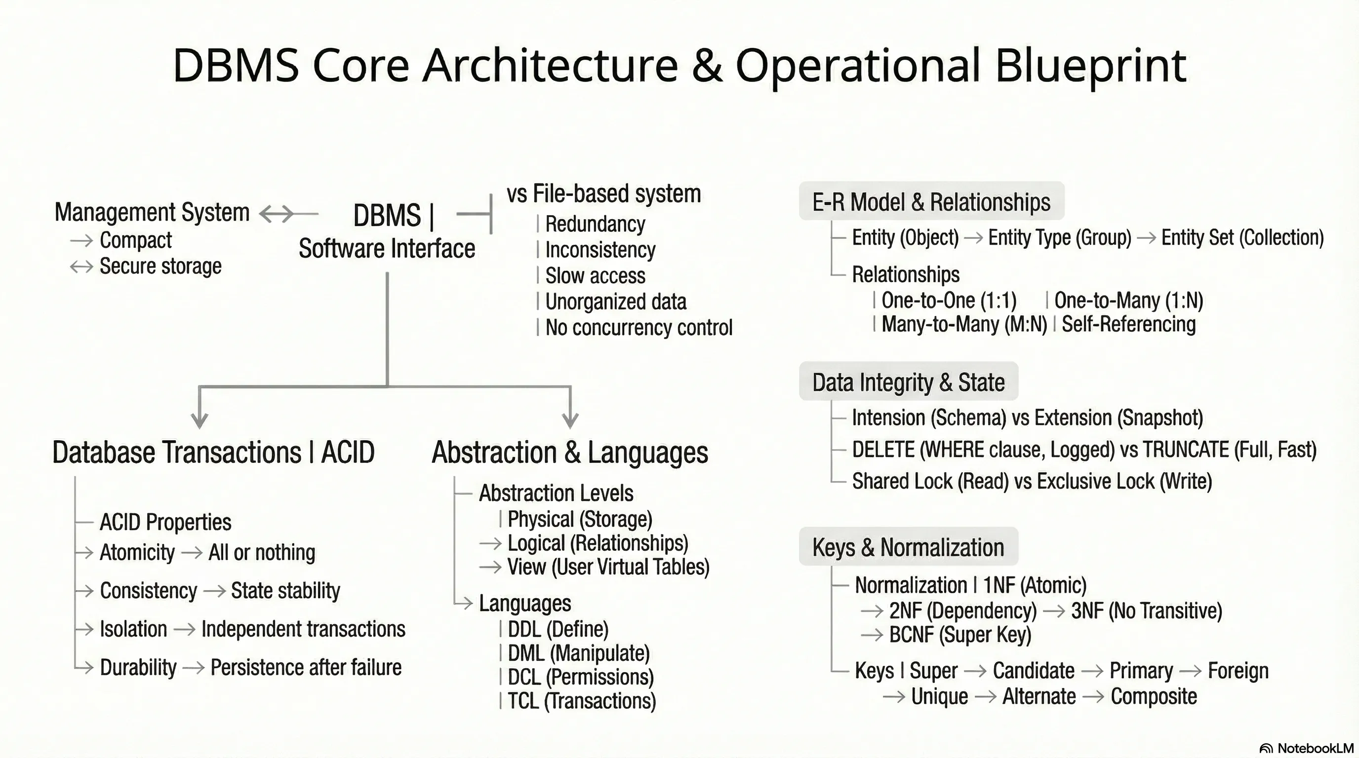
DBMS (Database Management System)

• Definition: A set of applications or programs that enable users to create and maintain a database.
• Utility:
  • Provides a tool or interface for performing various operations such as inserting, deleting, updating, etc., into a database.
  • Enables the storage of data more compactly and securely compared to a file-based system.
  • Helps users overcome problems like data inconsistency and data redundancy in a database.
  • Makes using a database more convenient and organized.
• Examples: File systems, XML, Windows Registry, etc.

RDBMS (Relational Database Management System)

• Definition: Introduced in the 1970s to access and store data more efficiently than DBMS.
• Structure: Stores data in the form of tables (rows and columns) compared to DBMS which stores data as files.
• Utility: Storing data as rows and columns makes it easier to locate specific values in the database and makes it more efficient compared to DBMS.
• Examples: MySQL, Oracle DB, etc.

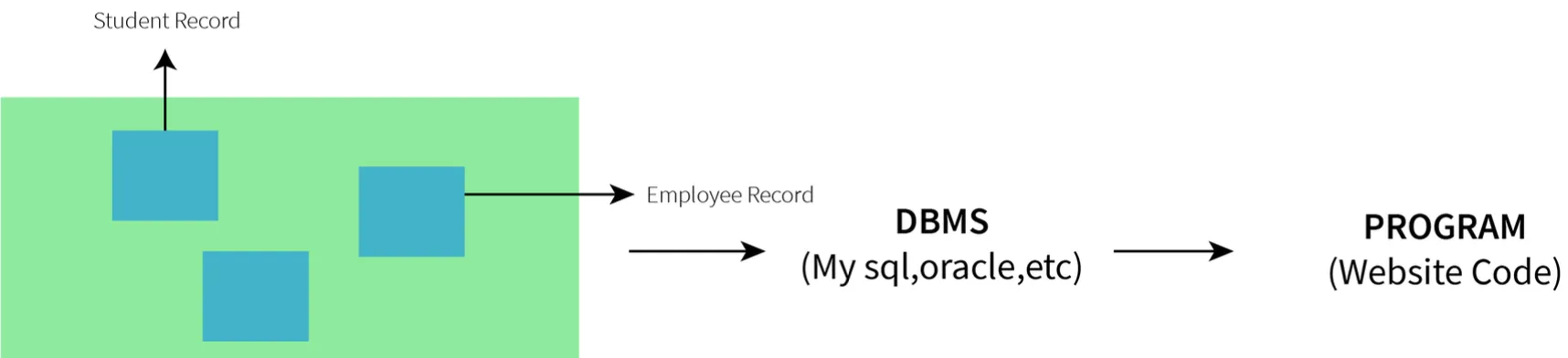
2. What is meant by a database?

• Definition: An organized, consistent, and logical collection of data that can easily be updated, accessed, and managed.
• Content: Mostly contains sets of tables or objects.
  • Object: Anything created using the create command is a database object.
  • Records and Fields: Tables consist of these.
• Tuple/Row: Represents a single entry in a table.
• Attribute/Column: Represents the basic units of data storage, containing information about a particular aspect of the table.
• Extraction: DBMS extracts data from a database in the form of queries given by the user.

3. Mention the issues with traditional file-based systems that make DBMS a better choice?

• Absence of Indexing: Leaves the only option of scanning the full page, making access to content tedious and super slow.
• Redundancy and Inconsistency: Files have many duplicate and redundant data; changing one makes all of them inconsistent.
• Data Access: Accessing data is harder because data is unorganized.
• Lack of Concurrency Control: Leads to one operation locking the entire page, whereas DBMS allows multiple operations on a single file simultaneously.
• Other Issues:
  • Integrity check issues
  • Data isolation issues
  • Atomicity issues
  • Security issues

4. Explain a few advantages of a DBMS.

• Data Sharing: Data from a single database can be simultaneously shared by multiple users. This enables end-users to react to changes quickly in the database environment.
• Integrity Constraints: The existence of these constraints allows storing data in an organized and refined manner.
• Controlling Redundancy: Eliminates redundancy by providing a mechanism that integrates all data in a single database.
• Data Independence: Allows changing the data structure without altering the composition of any executing application programs.
• Backup and Recovery: Can be configured to automatically create a backup of data and restore it whenever required.
• Data Security: Provides necessary tools to make storage and transfer reliable and secure.
  • Authentication: The process of giving restricted access to a user.
  • Encryption: Encrypting sensitive data such as OTP, credit card information, etc.

5. Explain different languages present in DBMS.

DDL (Data Definition Language)

• Contains commands required to define the database.
• Examples:

  CREATE, ALTER, DROP, TRUNCATE, RENAME
  

DML (Data Manipulation Language)

• Contains commands required to manipulate the data present in the database.
• Examples:

  SELECT, UPDATE, INSERT, DELETE
  

DCL (Data Control Language)

• Contains commands required to deal with user permissions and controls of the database system.
• Examples:

  GRANT, REVOKE
  

TCL (Transaction Control Language)

• Contains commands required to deal with the transaction of the database.
• Examples:

  COMMIT, ROLLBACK, SAVEPOINT
  

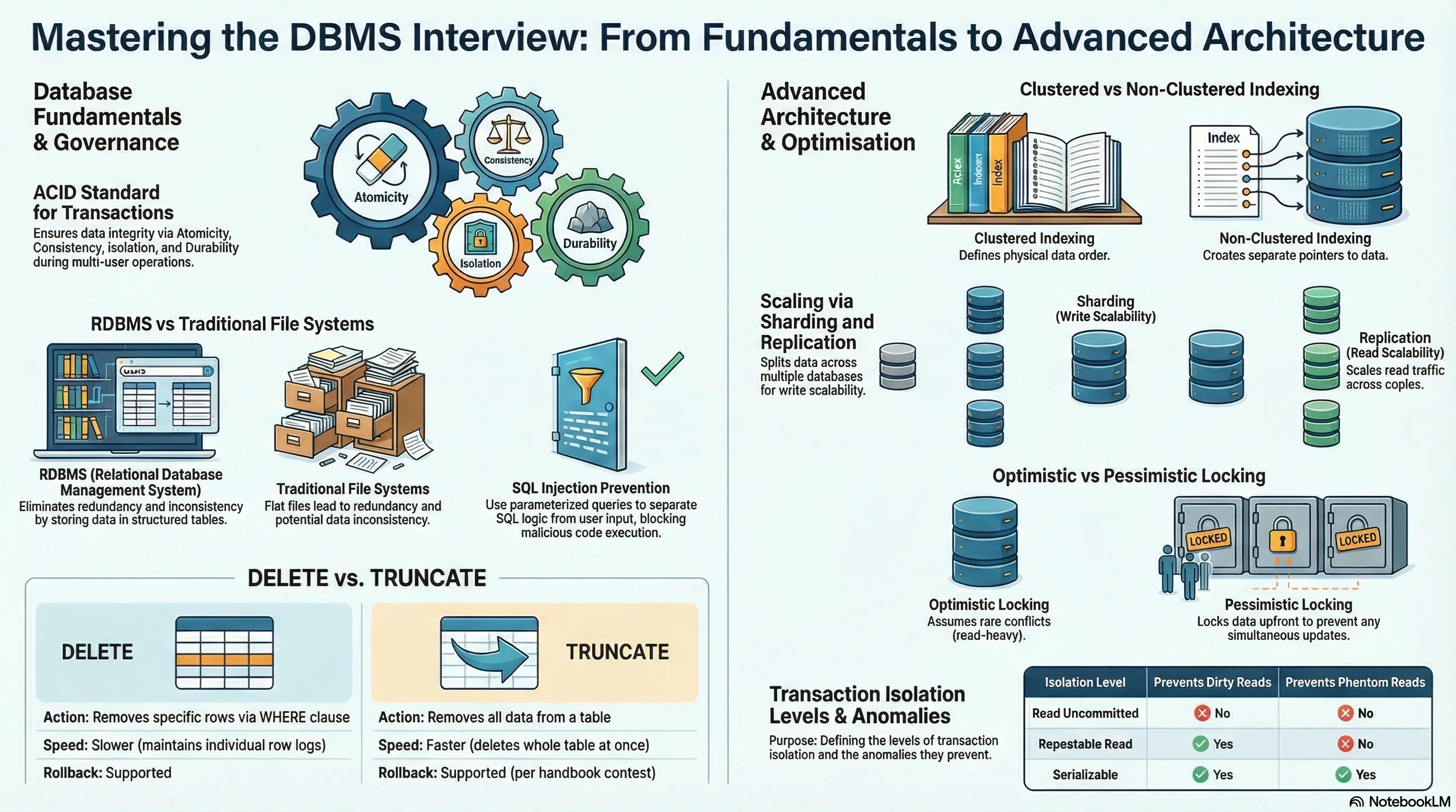
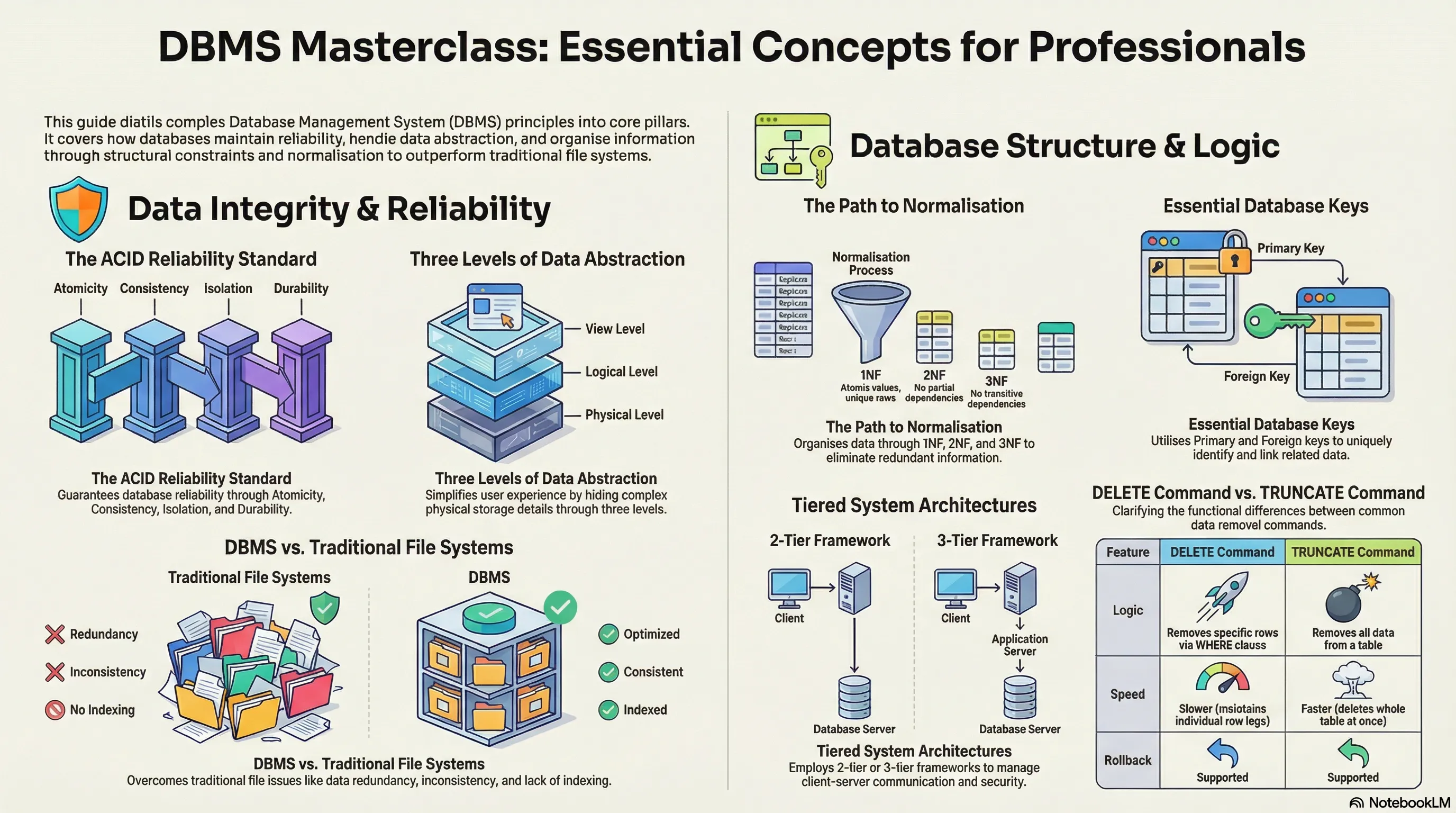
6. What is meant by ACID properties in DBMS?

ACID properties ensure a safe and secure way of sharing data among multiple users.

• A - Atomicity:
  • Reflects the concept of either executing the whole query or executing nothing at all.
  • If an update occurs, it should either be reflected in the whole database or not reflected at all.
  • In this Example
    • 
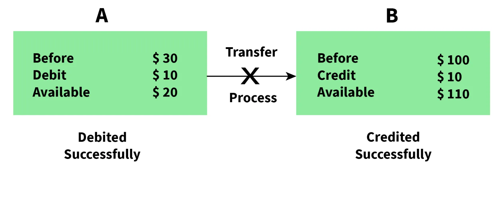
      • Partial Execution
      • No Atomicity
      • Execution Termination
  • In this Example
    • 
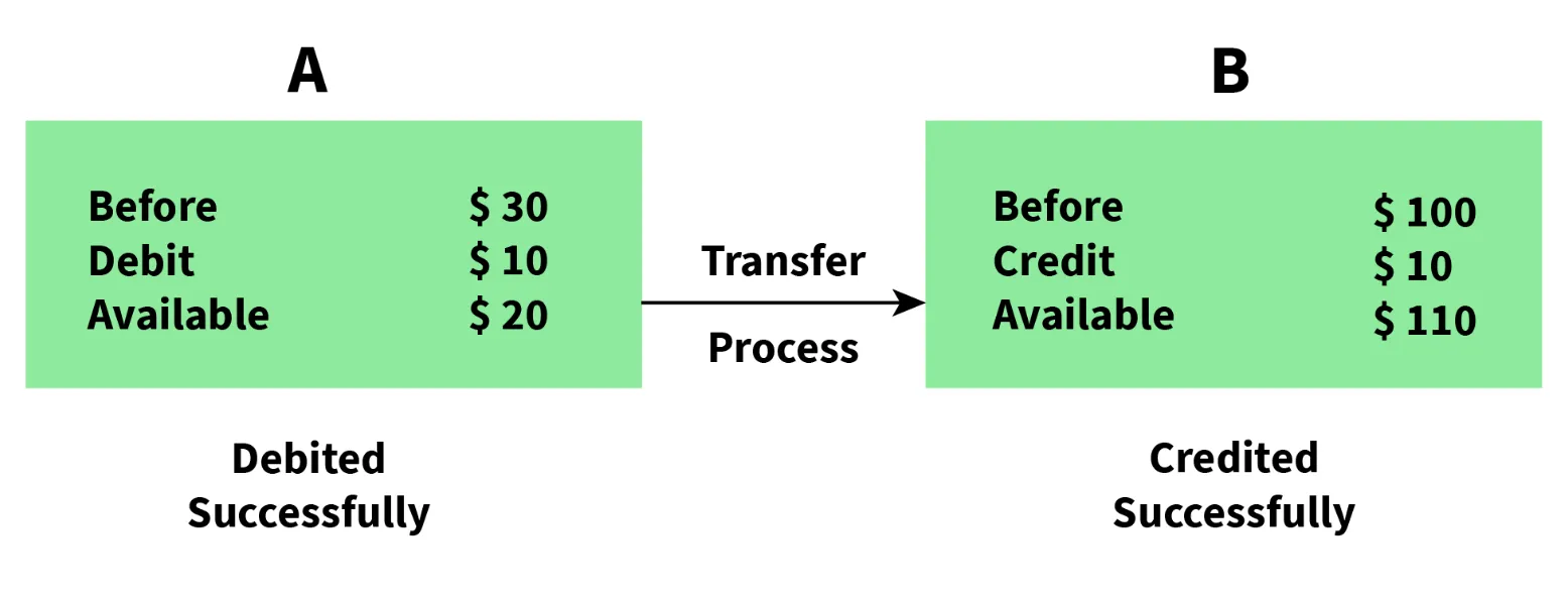
      • Complete Execution
      • Atomicity
      • Execution Successfull
• C - Consistency:
  • Ensures that data remains consistent before and after a transaction.
  • In this Example
    • 
      • Data is Consistent
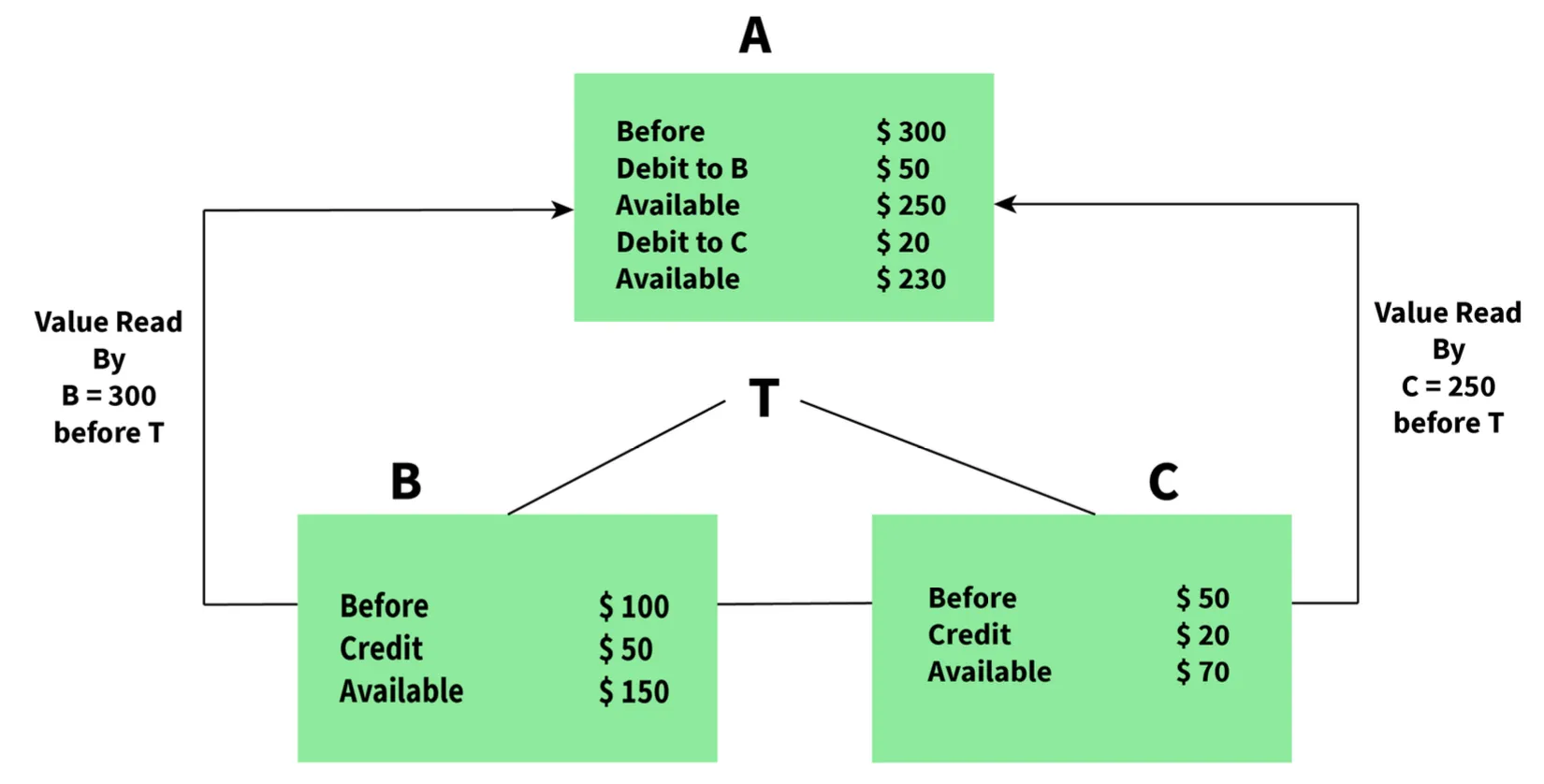
• I - Isolation:
  • Ensures each transaction occurs independently of others.
  • The state of an ongoing transaction does not affect the state of another ongoing transaction.
  • In this Example
    • 
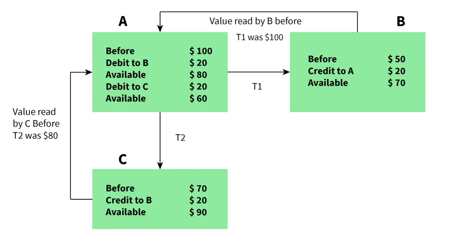
      • Isolation, Independent Execution T1 and T2 by A
• D - Durability:
  • Ensures data is not lost in cases of system failure or restart.
  • Data is present in the same state as it was before the failure/restart.

flowchart LR
    Start([Transaction Start]) --> A{Atomicity Check}
    A -->|All Operations| C{Consistency Check}
    A -->|Partial Failure| Rollback[Rollback All]
    C -->|Valid State| I[Isolation Applied]
    C -->|Invalid State| Rollback
    I --> Execute[Execute Transaction]
    Execute --> D[Durability Ensured]
    D --> Commit([Commit Success])
    Rollback --> Abort([Transaction Aborted])
    style Start fill:#2d3748,stroke:#4a90e2,color:#fff
    style Commit fill:#276749,stroke:#48bb78,color:#fff
    style Abort fill:#742a2a,stroke:#f56565,color:#fff
    style A fill:#1e3a5f,stroke:#4a90e2,color:#fff
    style C fill:#1e3a5f,stroke:#4a90e2,color:#fff
    style I fill:#2c5282,stroke:#4a90e2,color:#fff
    style Execute fill:#2c5282,stroke:#4a90e2,color:#fff
    style D fill:#2c5282,stroke:#4a90e2,color:#fff
    style Rollback fill:#742a2a,stroke:#f56565,color:#fff

7. Are NULL values in a database the same as that of blank space or zero?

• No, a NULL value is very different from zero and blank space.
• NULL: Represents a value that is assigned, unknown, unavailable, or not applicable.
• Blank Space: Represents a character.
• Zero: Represents a number.
• Example: A NULL value in "number_of_courses" means the value is unknown, whereas 0 means the student has not taken any courses.

---

Intermediate DBMS Interview Questions

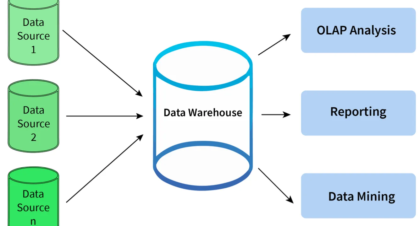
8. What is meant by Data Warehousing?

• Definition: The process of collecting, extracting, transforming, and loading data from multiple sources and storing them into one database.
• Function:
  • Acts as a central repository where data flows from transactional systems and other relational databases.
  • Used for data analytics.
  • Comprises a wide variety of an organization’s historical data.
  • Supports the decision-making process in an organization.

    flowchart LR
        S1[(Transactional DB)] --> Extract[Extract]
        S2[(Relational DB)] --> Extract
        S3[(External Sources)] --> Extract
        Extract --> Transform[Transform]
        Transform --> Load[Load]
        Load --> DW[(Data Warehouse)]
        DW --> Analytics[Data Analytics]
        Analytics --> Decision[Decision Making]
        style S1 fill:#1a365d,stroke:#4a90e2,color:#fff
        style S2 fill:#1a365d,stroke:#4a90e2,color:#fff
        style S3 fill:#1a365d,stroke:#4a90e2,color:#fff
        style Extract fill:#2c5282,stroke:#4a90e2,color:#fff
        style Transform fill:#2c5282,stroke:#4a90e2,color:#fff
        style Load fill:#2c5282,stroke:#4a90e2,color:#fff
        style DW fill:#1e3a5f,stroke:#4a90e2,color:#fff
        style Analytics fill:#2d3748,stroke:#4a90e2,color:#fff
        style Decision fill:#276749,stroke:#48bb78,color:#fff

9. Explain different levels of data abstraction in a DBMS.

Data abstraction is the process of hiding irrelevant details from users. It is divided into 3 levels:

1. Physical Level:
   • The lowest level, managed by DBMS.
   • Consists of data storage descriptions.
   • Details are typically hidden from system admins, developers, and users.
2. Conceptual or Logical Level:
   • Level on which developers and system admins work.
   • Determines what data is stored and the relationships between data points.
3. External or View Level:
   • Describes only part of the database.
   • Hides details of table schema and physical storage from users.
   • Example: The result of a query is View level data abstraction. A view is a virtual table created by selecting fields from one or more tables.

flowchart TB
    subgraph External["External/View Level"]
        V1[View 1]
        V2[View 2]
        V3[View N]
    end
    subgraph Conceptual["Conceptual/Logical Level"]
        L1[Tables & Relationships]
        L2[Schema Definitions]
    end
    subgraph Physical["Physical Level"]
        P1[Data Storage]
        P2[File Structures]
        P3[Indexing]
    end
    V1 --> L1
    V2 --> L1
    V3 --> L2
    L1 --> P1
    L2 --> P2
    L2 --> P3
    style External fill:#1e3a5f,stroke:#4a90e2,color:#fff
    style Conceptual fill:#2c5282,stroke:#4a90e2,color:#fff
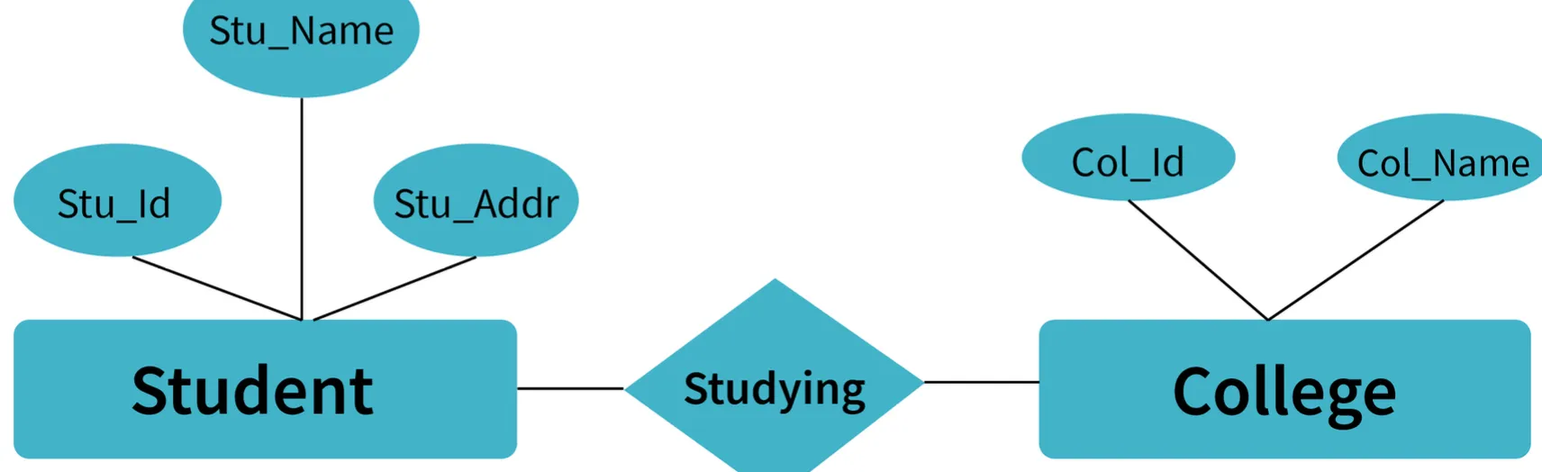
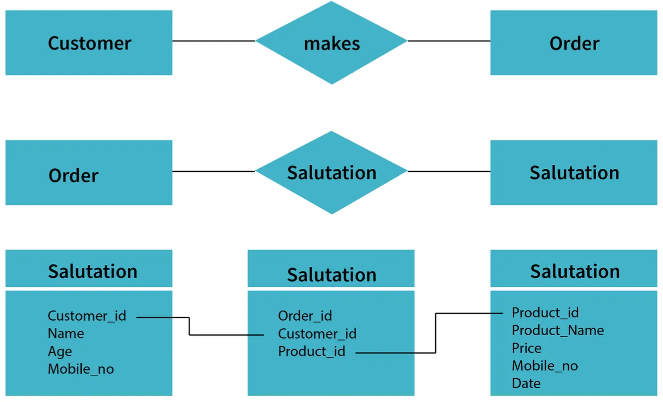
    style Physical fill:#1a365d,stroke:#4a90e2,color:#fff

10. What is meant by an entity-relationship (E-R) model? Explain the terms Entity, Entity Type, and Entity Set in DBMS.

• E-R Model: A diagrammatic approach to database design where real-world objects are represented as entities and relationships between them are mentioned.

Terms:

• Entity: A real-world object having attributes that represent characteristics of that particular object.
  • Example: A student, an employee, or a teacher.
• Entity Type: A collection of entities that have the same attributes.
  • One or more related tables in a database represent an entity type.
  • Attributes uniquely identify the entity.
  • Example: A student entity type has attributes like student_id, student_name, etc.
• Entity Set: A set of all the entities present in a specific entity type in a database.
  • Example: A set of all students, employees, teachers, etc.

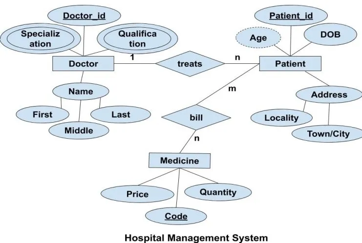
Example: Student Management System Sample

Example: Hospital Management System Sample

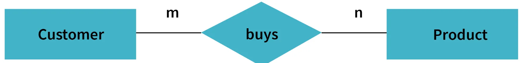
11. Explain different types of relationships amongst tables in a DBMS.

• One to One Relationship: Applied when a particular row in table X is linked to a singular row in table Y.
  • 
• One to Many Relationship: Applied when a single row in table X is related to many rows in table Y.
  • 
• Many to Many Relationship: Applied when multiple rows in table X can be linked to multiple rows in table Y.
  • 
• Self Referencing Relationship: Applied when a particular row in table X is associated with the same table.
  • 

erDiagram
    USER ||--|| PROFILE : "One-to-One"
    USER {
        int userId PK
        string name
    }
    PROFILE {
        int profileId PK
        int userId FK
        string bio
    }

    CUSTOMER ||--o{ ORDER : "One-to-Many"
    CUSTOMER {
        int customerId PK
        string customerName
    }
    ORDER {
        int orderId PK
        int customerId FK
        date orderDate
    }

    STUDENT }o--o{ COURSE : "Many-to-Many"
    STUDENT {
        int studentId PK
        string studentName
    }
    COURSE {
        int courseId PK
        string courseName
    }

    EMPLOYEE ||--o{ EMPLOYEE : "Self-Referencing"
    EMPLOYEE {
        int employeeId PK
        string employeeName
        int managerId FK
    }

12. Explain the difference between intension and extension in a database.

• Intension (Database Schema):
  • Used to define the description of the database.
  • Specified during the design of the database.
  • Mostly remains unchanged.
• Extension (Snapshot):
  • The measure of the number of tuples present in the database at any given point in time.
  • Value keeps changing as tuples are created, updated, or destroyed.

13. Explain the difference between the DELETE and TRUNCATE command in a DBMS.

DELETE Command

• Needed to delete rows from a table based on the condition provided by the WHERE clause.
• Deletes only rows specified by the WHERE clause.
• Can be rolled back if required.
• Maintains a log to lock the row of the table before deleting it; hence, it is slow.

TRUNCATE Command

• Needed to remove complete data from a table.
• Like a DELETE command with no WHERE clause.
• Removes complete data from a table.
• Can be rolled back even if required.
• Does not maintain a log and deletes the whole table at once; hence, it is fast.

14. What is a lock? Explain the major difference between a shared lock and an exclusive lock during a transaction in a database.

• Lock: A mechanism to protect a shared piece of data from getting updated by two or more database users at the same time. When a single user/session acquires a lock, no other user/session can modify that data until the lock is released.

Shared Lock

• Required for reading a data item.
• Many transactions may hold a lock on the same data item.
• Multiple transactions are allowed to read data items.

Exclusive Lock

• Required for any transaction about to perform a write operation.
• Does not allow more than one transaction.
• Prevents inconsistency in the database.

stateDiagram-v2
    [*] --> Unlocked
    Unlocked --> SharedLock : Read Request
    Unlocked --> ExclusiveLock : Write Request
    SharedLock --> SharedLock : More Read Requests
    SharedLock --> Unlocked : All Reads Complete
    SharedLock --> Waiting : Write Request
    ExclusiveLock --> Unlocked : Write Complete
    Waiting --> ExclusiveLock : Shared Lock Released
    ExclusiveLock --> [*]

    note right of SharedLock
        Multiple transactions
        can read simultaneously
    end note

    note right of ExclusiveLock
        Only one transaction
        can write at a time
    end note

15. What is meant by normalization and denormalization?

• Normalization:
  • A process of reducing redundancy by organizing data into multiple tables.
  • Leads to better usage of disk spaces.
  • Makes it easier to maintain database integrity.
• Denormalization:
  • The reverse process of normalization.
  • Combines tables which have been normalized into a single table.
  • Makes data retrieval faster.
  • JOIN operation allows creating a denormalized form by reversing normalization.

---

Advanced DBMS Interview Questions

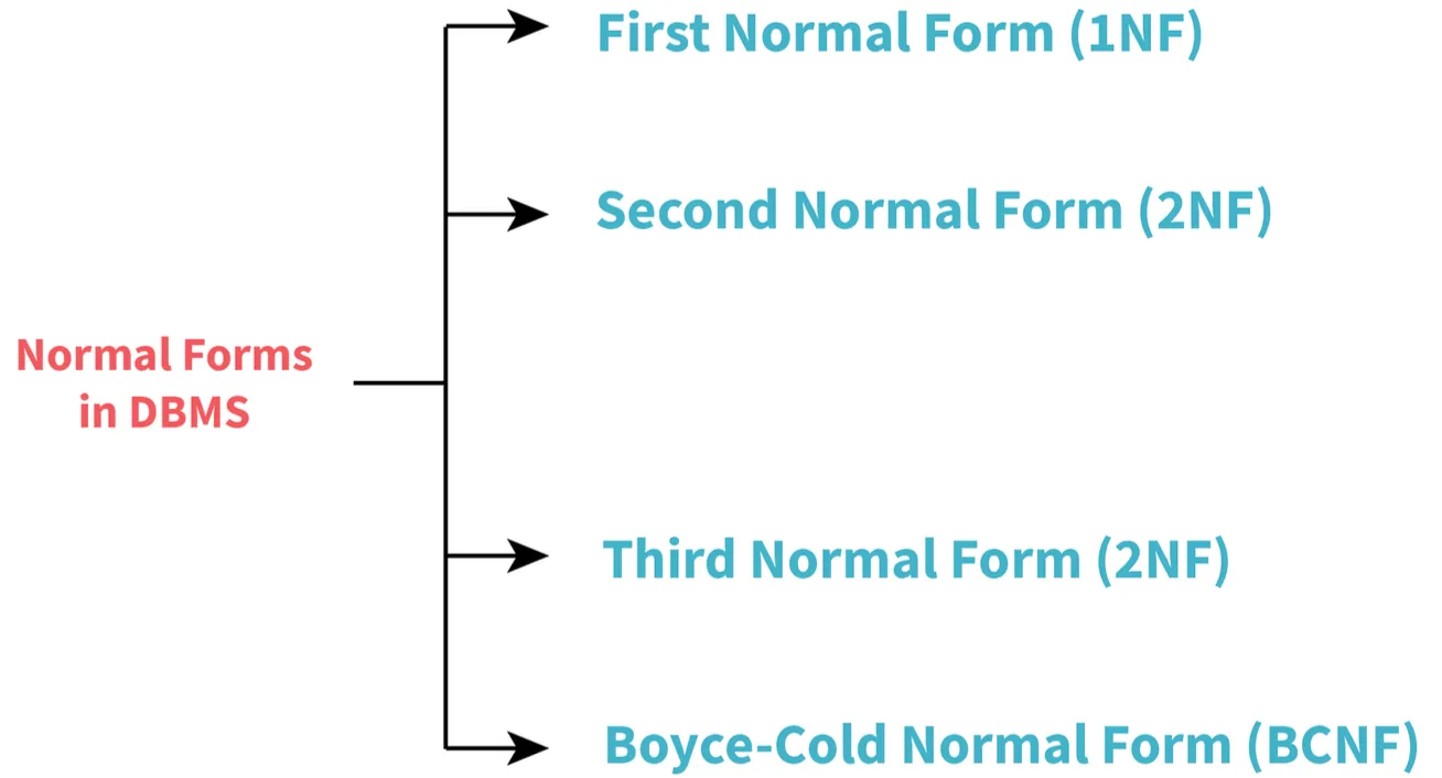
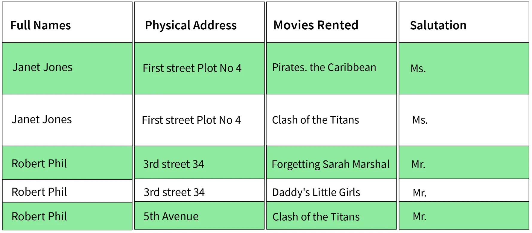
16. Explain different types of Normalization forms in a DBMS.

Reference Example Sample:

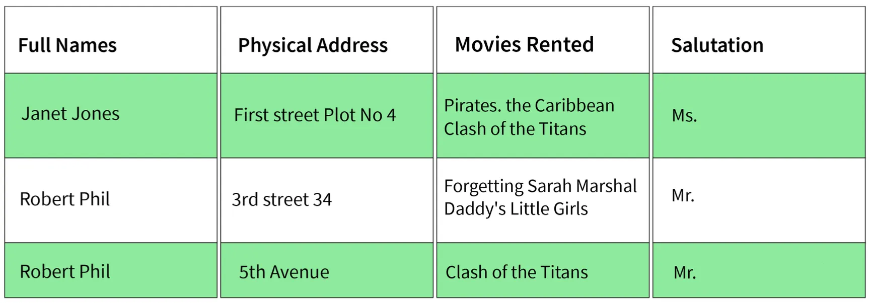
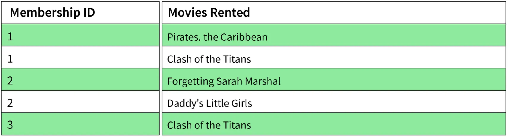
1. First Normal Form (1NF)

• Simplest type. Conditions:
  • Every column must have a single value and should be atomic.
  • Duplicate columns from the same table should be removed.
  • Separate tables should be created for each group of related data.
  • Each row should be identified with a unique column.

Sample's 1NF form:

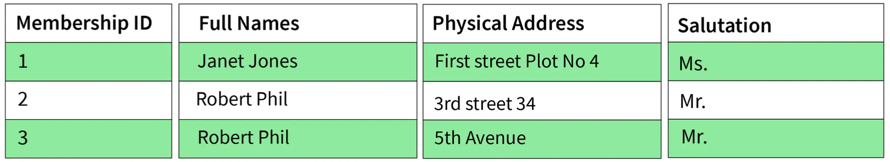
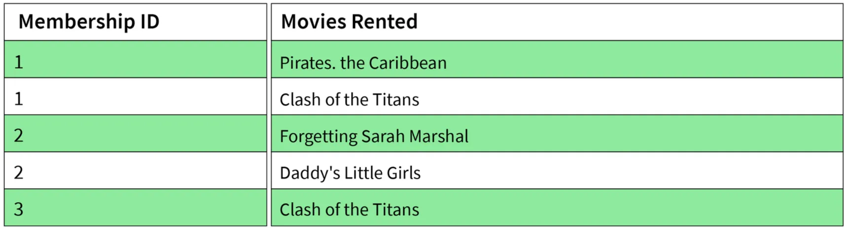
2. Second Normal Form (2NF)

• Conditions:
  • Table must be in 1NF.
  • Every non-prime attribute should be fully functionally dependent on the primary key.
  • Explanation: Every non-key attribute must depend on the primary key such that if any key element is deleted, the non-key element will be saved.

Sample's 2NF form:

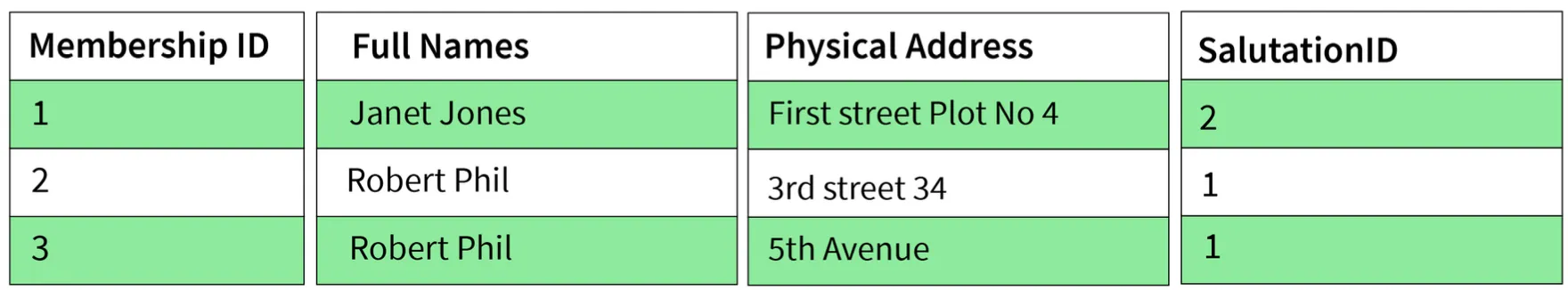
3. Third Normal Form (3NF)

• Conditions:
  • Table must be in 2NF.
  • There is no transitive functional dependency of one attribute on any attribute in the same table.

Sample's 3NF form:

4. Boyce-Codd Normal Form (BCNF) / 3.5NF

• Advanced form of 3NF. Conditions:
  • Table must be in 3NF.
  • For every functional dependency A -> B, A should be the super key of the table.
  • Implication: A can't be a non-prime attribute if B is a prime attribute.

flowchart LR
    Unnormalized[Unnormalized Data] --> 1NF
    1NF["1NF<br/>Atomic Values<br/>Unique Rows"] --> 2NF
    2NF["2NF<br/>1NF +<br/>Full Functional Dependency"] --> 3NF
    3NF["3NF<br/>2NF +<br/>No Transitive Dependency"] --> BCNF
    BCNF["BCNF<br/>3NF +<br/>Determinant is Super Key"]
    style Unnormalized fill:#742a2a,stroke:#f56565,color:#fff
    style 1NF fill:#2c5282,stroke:#4a90e2,color:#fff
    style 2NF fill:#2c5282,stroke:#4a90e2,color:#fff
    style 3NF fill:#2c5282,stroke:#4a90e2,color:#fff
    style BCNF fill:#276749,stroke:#48bb78,color:#fff

17. Explain different types of keys in a database.

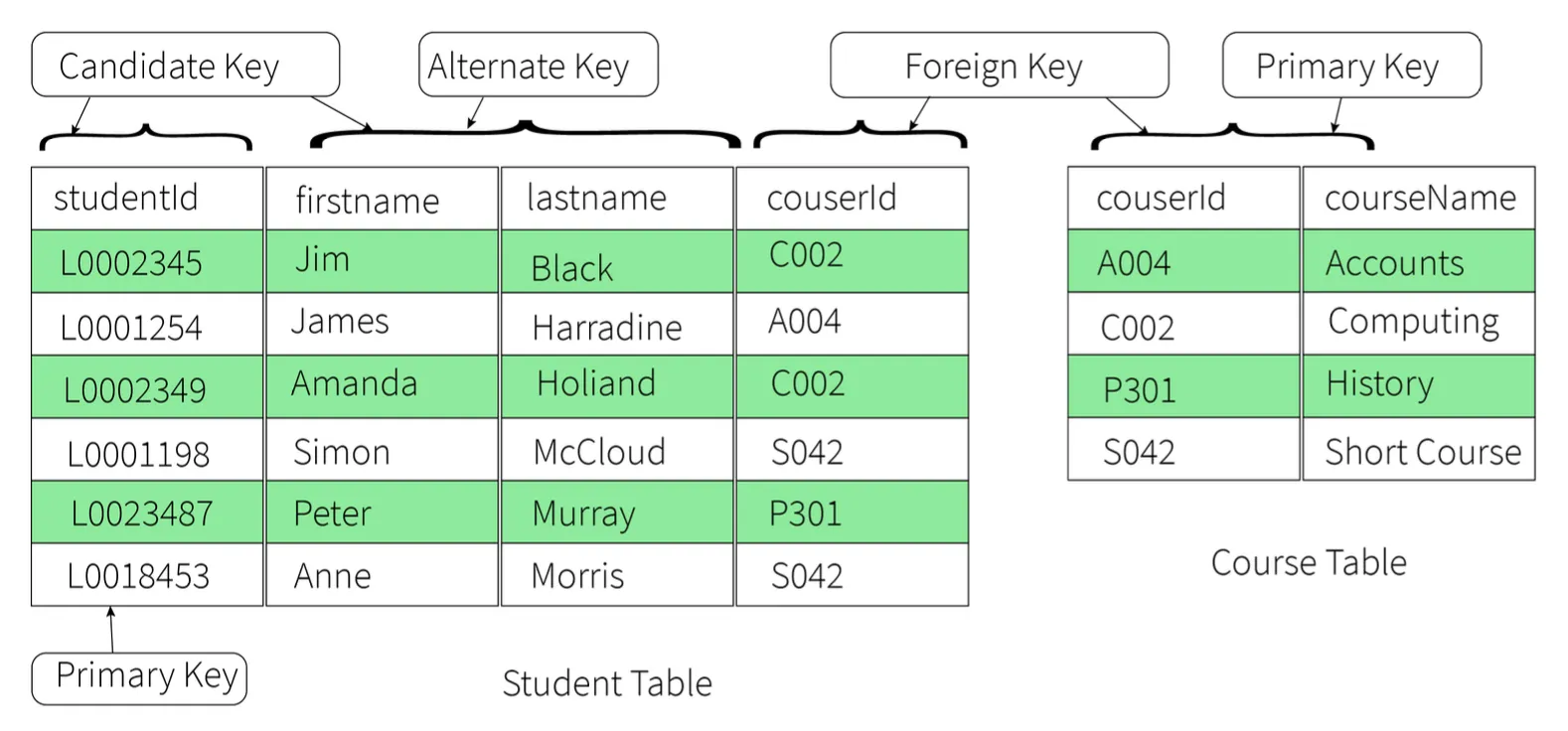
1. Candidate Key

• A set of properties that can uniquely identify a table.
• Each table may have multiple candidate keys.
• One key amongst them is chosen as the primary key.
• Example: studentId and firstName can both be Candidate Keys if they uniquely identify every tuple.

2. Super Key

• A set of attributes that can uniquely identify a tuple.
• Candidate key and primary key are subsets of the super key (the super key is their superset).

3. Primary Key

• A set of attributes used to uniquely identify every tuple.
• Chosen from the candidate keys.
• Does not allow NULL values.
• Example: studentId chosen over firstName for the student table.

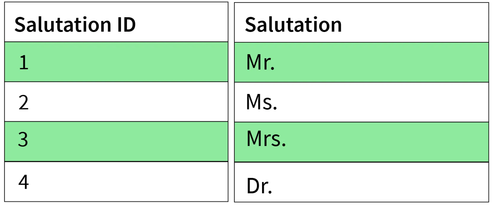
4. Unique Key

• Similar to primary key but allows NULL values in the column.
• Essentially primary keys with NULL values.

5. Alternate Key

• All candidate keys not chosen as primary keys.
• Example: If studentId is Primary, firstName and lastname are alternate keys.

6. Foreign Key

• An attribute that can only take values present in one table common to the attribute present in another table.
• Example: courseId in the Student table is a foreign key to the Course table.

7. Composite Key

• A combination of two or more columns that can uniquely identify each tuple in a table.
• Example: Grouping studentId and firstname.

flowchart TB
    SK[Super Key<br/>All Possible Combinations] --> CK
    CK[Candidate Key<br/>Minimal Super Key] --> PK
    CK --> AK
    PK[Primary Key<br/>Selected Candidate<br/>No NULL] --> UK
    AK[Alternate Key<br/>Non-selected Candidates]
    UK[Unique Key<br/>Like Primary<br/>Allows NULL]
    FK[Foreign Key<br/>References Primary Key<br/>in Another Table]
    COMP[Composite Key<br/>Multiple Columns Combined]
    style SK fill:#1a365d,stroke:#4a90e2,color:#fff
    style CK fill:#2c5282,stroke:#4a90e2,color:#fff
    style PK fill:#276749,stroke:#48bb78,color:#fff
    style AK fill:#2c5282,stroke:#4a90e2,color:#fff
    style UK fill:#2c5282,stroke:#4a90e2,color:#fff
    style FK fill:#744210,stroke:#ed8936,color:#fff
    style COMP fill:#2d3748,stroke:#4a90e2,color:#fff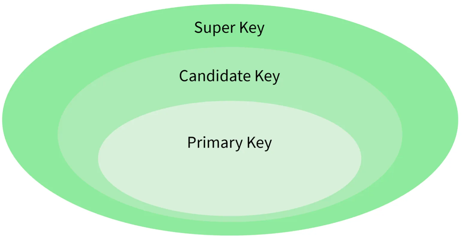

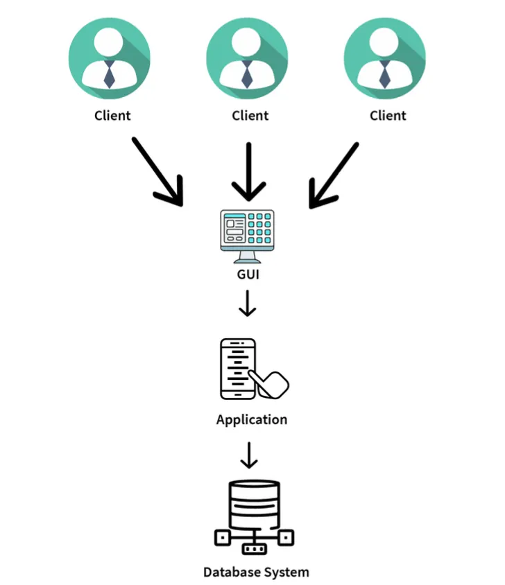
18. Explain the difference between a 2-tier and 3-tier architecture in a DBMS.

2-Tier Architecture

• Client-Server architecture.
• Applications at the client end directly communicate with the database at the server end.
• No middleware involved.
• Examples: Contact Management System created using MS-Access, Railway Reservation System.

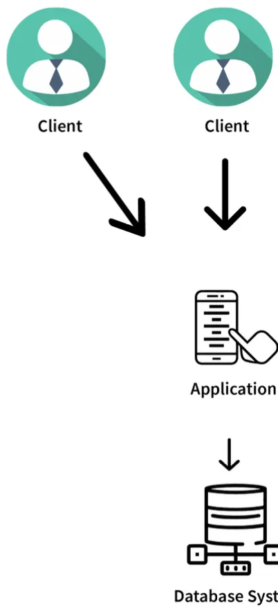
3-Tier Architecture

• Contains another layer (Middleware) between the client and the server.
• Provides GUI to users.
• Makes the system much more secure and accessible.
• Flow: Client Application <-> Server Application <-> Database System.
• Examples: Designing registration forms (text box, label, button), large websites on the Internet.

flowchart TB
    subgraph TwoTier["2-Tier Architecture"]
        C1[Client Application<br/>Presentation + Business Logic]
        D1[(Database Server<br/>Data Layer)]
        C1 --> D1
        D1 --> C1
    end

    subgraph ThreeTier["3-Tier Architecture"]
        C2[Client Application<br/>Presentation Layer]
        M[Middleware / Application Server<br/>Business Logic Layer]
        D2[(Database Server<br/>Data Layer)]
        C2 --> M
        M --> C2
        M --> D2
        D2 --> M
    end

    style C1 fill:#2c5282,stroke:#4a90e2,color:#fff
    style D1 fill:#1a365d,stroke:#4a90e2,color:#fff
    style C2 fill:#2c5282,stroke:#4a90e2,color:#fff
    style M fill:#744210,stroke:#ed8936,color:#fff
    style D2 fill:#1a365d,stroke:#4a90e2,color:#fff
    style TwoTier fill:#1e293b,stroke:#4a90e2,color:#fff
    style ThreeTier fill:#1e293b,stroke:#4a90e2,color:#fff

---

---

DBMS Indexing & Query Optimization

19. What is selectivity/cardinality and why does it matter for indexing?

• Selectivity refers to how unique the values in a column are.
• High selectivity means most values are unique (e.g., user IDs). Low selectivity means many rows share the same value (e.g., status flags).
• Indexes work best on high-selectivity columns. Indexing low-selectivity columns often gives little benefit.
• Understanding data distribution helps decide which columns should be indexed.

20. What is an index and why can indexing slow down INSERT/UPDATE/DELETE?

• An index is a data structure that helps the database find rows faster without scanning the full table.
• It improves read performance by reducing the amount of data searched.
• However, every time you insert, update, or delete data, the index also needs to be updated.
• This extra write overhead slows down write operations. The more indexes a table has, the slower writes become.
• Indexing is always a balance between read speed and write performance.

21. Difference between clustered and non-clustered index

• Clustered Index: Defines the physical order of data in the table. A table can have only one clustered index. Faster for range queries.
• Non-Clustered Index: Stores a separate structure that points to the actual rows. Does not change how data is stored on disk. Better for specific lookups.
• Choosing the wrong type can lead to inefficient queries.

flowchart LR
    subgraph CI["Clustered Index"]
        direction TB
        CD[(Table Data\nordered by index key)] --> CR1[Row 1: id=1]
        CD --> CR2[Row 2: id=2]
        CD --> CR3[Row 3: id=3]
    end
    subgraph NCI["Non-Clustered Index"]
        direction TB
        NI[Index Structure\nsorted by key] --> P1[Pointer → Row A]
        NI --> P2[Pointer → Row B]
        NI --> P3[Pointer → Row C]
        P1 --> ND[(Table Data\nunordered)]
        P2 --> ND
        P3 --> ND
    end
    style CI fill:#1e3a5f,stroke:#4a90e2,color:#fff
    style NCI fill:#1a365d,stroke:#4a90e2,color:#fff
    style CD fill:#2c5282,stroke:#4a90e2,color:#fff
    style ND fill:#2c5282,stroke:#4a90e2,color:#fff
    style NI fill:#744210,stroke:#ed8936,color:#fff

22. When does a query not use an index even if one exists?

• The query optimizer thinks a full table scan is faster (e.g., when a large percentage of rows match the condition).
• Using functions on indexed columns can prevent index usage.
• Mismatched data types or implicit conversions can break index access.
• Poorly written queries confuse the optimizer.

23. What is a composite index and the leftmost prefix rule?

• A composite index is an index created on multiple columns together.
• The leftmost prefix rule means the index is used only if the query filters starting from the first column.
• Example: An index on (user_id, order_date) works for queries filtering by user_id, but not for queries filtering only by order_date.
• Always match index column order with real query usage.

flowchart TD
    IDX["Composite Index\n(user_id, order_date, amount)"]
    IDX --> Q1["WHERE user_id = 5\n✅ Uses index"]
    IDX --> Q2["WHERE user_id = 5\nAND order_date = '2024-01-01'\n✅ Uses index"]
    IDX --> Q3["WHERE user_id = 5\nAND order_date = '2024-01-01'\nAND amount > 100\n✅ Uses index"]
    IDX --> Q4["WHERE order_date = '2024-01-01'\n❌ Skips index\n(no leftmost prefix)"]
    IDX --> Q5["WHERE amount > 100\n❌ Skips index\n(no leftmost prefix)"]
    style IDX fill:#744210,stroke:#ed8936,color:#fff
    style Q1 fill:#276749,stroke:#48bb78,color:#fff
    style Q2 fill:#276749,stroke:#48bb78,color:#fff
    style Q3 fill:#276749,stroke:#48bb78,color:#fff
    style Q4 fill:#742a2a,stroke:#f56565,color:#fff
    style Q5 fill:#742a2a,stroke:#f56565,color:#fff

24. What is a covering index and how does it reduce table lookups?

• A covering index contains all the columns needed by a query.
• This allows the database to fetch results directly from the index without accessing the table, resulting in fewer disk reads.
• Especially useful for read-heavy/reporting queries.
• Trade-off: They increase index size and slow down writes.

25. What is an execution plan and what do you check first?

• An execution plan shows how the database executes a query step by step — which indexes are used, how tables are joined, etc.
• First checks:
  • Are indexes being used or ignored?
  • Are there full table scans on large tables?
  • What are the estimated vs actual row counts?
• A bad execution plan usually points to missing or incorrect indexes.

flowchart TD
    Q([Run Query]) --> EP[Get Execution Plan]
    EP --> C1{Index Used?}
    C1 -->|Yes| C2{Full Table Scan\non Large Table?}
    C1 -->|No| Fix1[Add or Fix Index]
    C2 -->|No| C3{Estimated vs Actual\nRow Count Match?}
    C2 -->|Yes| Fix2[Rewrite Query or\nAdd Index]
    C3 -->|Yes| OK([Plan is Healthy])
    C3 -->|No| Fix3[Update Statistics\nor Rewrite Query]
    style Q fill:#2d3748,stroke:#4a90e2,color:#fff
    style EP fill:#2c5282,stroke:#4a90e2,color:#fff
    style OK fill:#276749,stroke:#48bb78,color:#fff
    style Fix1 fill:#742a2a,stroke:#f56565,color:#fff
    style Fix2 fill:#742a2a,stroke:#f56565,color:#fff
    style Fix3 fill:#744210,stroke:#ed8936,color:#fff

26. Index scan vs index seek and when they occur

• Index Seek: The database jumps directly to matching rows using the index. Fast and efficient. Indicates good indexing and selective filters.
• Index Scan: The database scans a large part or all of the index. Happens when many rows match the condition.
• Frequent scans on large datasets can hurt performance.

flowchart LR
    subgraph Seek["Index Seek ✅ (Fast)"]
        direction TB
        SK1[Index Root] --> SK2[Branch Node]
        SK2 --> SK3[Target Leaf]
        SK3 --> SK4["Matching Row\n(Direct Jump)"]
    end
    subgraph Scan["Index Scan ⚠️ (Slower)"]
        direction TB
        SC1[Index Start] --> SC2[Leaf 1]
        SC2 --> SC3[Leaf 2]
        SC3 --> SC4[Leaf 3]
        SC4 --> SC5["... N Leaves\n(Full Traversal)"]
    end
    style Seek fill:#1e3a5f,stroke:#48bb78,color:#fff
    style Scan fill:#1e293b,stroke:#ed8936,color:#fff
    style SK4 fill:#276749,stroke:#48bb78,color:#fff
    style SC5 fill:#744210,stroke:#ed8936,color:#fff

27. What is index fragmentation or bloat and its impact?

• Index fragmentation happens when index pages become disorganized over time due to frequent inserts, updates, and deletes.
• Fragmented indexes require more disk reads, causing query performance to slowly degrade.
• Fix: Rebuilding or reorganizing indexes. Regular maintenance is important for long-running production systems.

28. Common production reasons for slow queries and debugging flow

• Slow queries are often caused by missing indexes, bad joins, or large data growth.
• Debugging steps:
  1. Check query execution time and execution plans.
  2. Look for full scans, high I/O, or blocking locks.
  3. Tune indexes to fix most issues.
• Performance debugging is about data size, not just SQL syntax.

---

DBMS Security & Governance

29. Risk of giving apps superuser DB permissions

• Superuser access allows full control over the database.
• If an app is compromised, attackers gain unlimited power — leading to data loss or system damage.
• It also increases the impact of bugs or bad queries.
• Best practice: Production apps should never use superuser accounts. Limiting permissions reduces risk significantly.

30. What is SQL injection and how do parameterized queries prevent it?

• SQL Injection happens when user input is treated as part of a SQL command, allowing attackers to modify the query to access or change data.
• Parameterized queries separate SQL logic from user input — the database treats inputs only as values, not executable code.
• This completely blocks injection attacks and is the safest, most common defense.

flowchart TD
    subgraph Unsafe["❌ SQL Injection Vulnerable"]
        U1[User Input: '\' OR 1=1 --'] --> U2["Query: SELECT * FROM users\nWHERE name = '' OR 1=1 --'"]
        U2 --> U3["Returns ALL rows\n🔓 Data breach!"]
    end
    subgraph Safe["✅ Parameterized Query"]
        S1[User Input: '\' OR 1=1 --'] --> S2["Query: SELECT * FROM users\nWHERE name = ?"]
        S2 --> S3[DB treats input as literal value]
        S3 --> S4["Returns 0 rows\n🔒 Safe"]
    end
    style Unsafe fill:#742a2a,stroke:#f56565,color:#fff
    style Safe fill:#1e3a5f,stroke:#48bb78,color:#fff
    style U3 fill:#742a2a,stroke:#f56565,color:#fff
    style S4 fill:#276749,stroke:#48bb78,color:#fff

31. DB authentication vs authorization and roles in practice

• Authentication: Checks who you are (username/password).
• Authorization: Decides what actions you are allowed to perform.
• Roles group permissions (read, write, admin) and are assigned to users instead of individual privileges.
• This makes access easier to manage and audit.

32. What is row-level security and a real use-case?

• Row-level security restricts which rows a user can see in a table — the same query returns different results for different users.
• Use-case: Multi-tenant systems where each customer sees only their own data.
• The logic is enforced by the database itself, preventing accidental data leaks at the app layer.

33. Encryption at rest vs encryption in transit

• Encryption at Rest: Protects data stored on disk. Prevents data theft if disks or backups are accessed.
• Encryption in Transit: Protects data moving between the app and database (e.g., using TLS/SSL).
• Both are required for full security — one does not replace the other.

flowchart LR
    App[Application] -->|TLS/SSL Encrypted\nEncryption in Transit| DB[(Database Server)]
    DB -->|Encrypted at Rest\non disk & backups| Disk[💾 Disk / Storage]
    style App fill:#2c5282,stroke:#4a90e2,color:#fff
    style DB fill:#1a365d,stroke:#4a90e2,color:#fff
    style Disk fill:#744210,stroke:#ed8936,color:#fff

34. How do you store DB credentials safely?

• DB credentials should never be hardcoded in source code.
• Stored in a secrets manager or secure vault; applications fetch credentials at runtime.
• Access is controlled using IAM or service identities.
• Secrets can be rotated without code changes, reducing the risk of leaks.

35. What does least privilege mean in DB access control?

• Least privilege means giving only the permissions strictly required.
• Applications should not have admin or schema-altering access; read-only users should not be able to write data.
• This limits damage if credentials are compromised and reduces the chance of human error.

36. What is auditing and what should be logged?

• Auditing tracks important actions performed in the database.
• What to log: Logins, permission changes, schema updates, and sensitive data access.
• Audit logs help in security investigations and compliance. They must be protected from tampering.

37. How do you protect PII data?

• PII can be protected using masking, tokenization, or encryption.
• Masking: Hides parts of the data for non-privileged users.
• Tokenization: Replaces sensitive values with safe references.
• Encryption: Protects data at rest and in backups.
• The goal is minimizing exposure by using the right technique for each access need.

---

DBMS SQL & Querying

38. Difference between WHERE and HAVING

• WHERE filters rows before any grouping or aggregation. It works on individual records and cannot use aggregate functions.
• HAVING is applied after GROUP BY and is meant for filtering aggregated results.
• Example: Filter orders by status → use WHERE. Filter customers with total orders > 5 → use HAVING.
• A good rule: filter early using WHERE whenever possible.

flowchart LR
    T[(Raw Table Rows)] --> W[WHERE Filter\nearly, row-by-row]
    W --> GB[GROUP BY]
    GB --> AGG[Aggregate\nCOUNT / SUM / AVG]
    AGG --> H[HAVING Filter\non aggregated results]
    H --> R([Result Set])
    style T fill:#1a365d,stroke:#4a90e2,color:#fff
    style W fill:#744210,stroke:#ed8936,color:#fff
    style GB fill:#2c5282,stroke:#4a90e2,color:#fff
    style AGG fill:#2c5282,stroke:#4a90e2,color:#fff
    style H fill:#6a1b9a,stroke:#ce93d8,color:#fff
    style R fill:#276749,stroke:#48bb78,color:#fff

39. INNER JOIN vs LEFT JOIN and when LEFT JOIN behaves like INNER JOIN

• INNER JOIN: Returns only rows that exist in both tables.
• LEFT JOIN: Returns all rows from the left table, even if there is no matching row on the right side.
• Gotcha: A LEFT JOIN can accidentally behave like an INNER JOIN if you add conditions on the right table in the WHERE clause (removes NULL rows). Fix: put right-table conditions inside the ON clause instead.

flowchart LR
    subgraph IJ["INNER JOIN"]
        direction LR
        LA([Table A]) --> AB([Matching Rows Only])
        LB([Table B]) --> AB
    end
    subgraph LJ["LEFT JOIN"]
        direction LR
        LL([All of Table A]) --> LJ2([Matched Rows])
        LL --> LN([Unmatched rows: NULL on right])
        LB2([Table B]) --> LJ2
    end
    style IJ fill:#1e3a5f,stroke:#4a90e2,color:#fff
    style LJ fill:#1a365d,stroke:#48bb78,color:#fff
    style AB fill:#2c5282,stroke:#4a90e2,color:#fff
    style LJ2 fill:#276749,stroke:#48bb78,color:#fff
    style LN fill:#2d3748,stroke:#4a90e2,color:#fff

40. What causes duplicate rows after a JOIN, and how to fix it

• Duplicate rows appear when one row in a table matches multiple rows in another (one-to-many relationships).
• Fixes:
  • Aggregate data before joining.
  • Ensure you are joining on the correct keys.
  • Use DISTINCT cautiously (it can hide real data issues).
• Understanding the data structure is more important than forcing uniqueness.

41. What is a correlated subquery, and when is it slower than a JOIN?

• A correlated subquery depends on values from the outer query and runs once for each row returned by the main query.
• Because of this repeated execution, it can be slow on large datasets.
• In many cases, the same logic can be rewritten using a JOIN, which executes more efficiently.
• Best avoided in high-volume production queries.

42. UNION vs UNION ALL from a performance viewpoint

• UNION: Combines results and removes duplicate rows. Requires extra sorting/comparison — slower.
• UNION ALL: Appends results without checking for duplicates — faster and uses fewer resources.
• If datasets do not overlap, always prefer UNION ALL.

flowchart TD
    Q1[Query 1 Results] --> U{UNION Type?}
    Q2[Query 2 Results] --> U
    U -->|UNION| SORT[Sort + Deduplicate\nExtra overhead ⚠️]
    U -->|UNION ALL| FAST[Direct Append\nNo deduplication ✅]
    SORT --> R1([Final Result\nNo duplicates])
    FAST --> R2([Final Result\nMay have duplicates])
    style U fill:#2c5282,stroke:#4a90e2,color:#fff
    style SORT fill:#744210,stroke:#ed8936,color:#fff
    style FAST fill:#276749,stroke:#48bb78,color:#fff
    style R1 fill:#2d3748,stroke:#4a90e2,color:#fff
    style R2 fill:#2d3748,stroke:#4a90e2,color:#fff

43. How to write Top-N per group queries

• Use window functions like ROW_NUMBER() with PARTITION BY to rank rows within each group, then filter the top N.
• Alternative: Use a correlated subquery comparing values within the same group (older databases).
• Window functions are clearer, faster, and easier to maintain in modern SQL.

44. What is a CTE and how it differs from a subquery

• A CTE (Common Table Expression), written using the WITH clause, is a temporary named result set used within a query.
• Makes complex queries easier to read and maintain compared to nested subqueries.
• CTEs can be referenced multiple times in the same query.
• Recursive CTEs handle hierarchical data (e.g., employee reporting structures).

45. What is a VIEW and when should you avoid it

• A view is a stored SQL query that behaves like a virtual table. It simplifies complex queries and provides consistent data access.
• Views do not store data — the underlying query runs every time the view is accessed.
• Avoid views for heavy calculations or frequently accessed large datasets, as they can hide inefficient SQL and make debugging harder.

46. What is a materialized view and its trade-offs

• A materialized view stores the actual result of a query, making read operations very fast — useful for reporting and analytics.
• Trade-offs: Data can become stale and needs to be refreshed (manually or on a schedule). Refreshing can be expensive.
• Best used when fast reads are more important than real-time accuracy.

---

Replication, Sharding & Distributed DB Concepts

47. What is partitioning or sharding and when should you shard?

• Sharding splits data across multiple databases based on a key, distributing reads and writes to improve scalability.
• Used when a single database can no longer handle the load or data size.
• Downsides: Increases system complexity; cross-shard queries become harder.
• Teams usually shard only after vertical scaling is no longer enough.

flowchart TD
    App[Application] --> Router[Shard Router / Proxy]
    Router -->|shard_key mod 3 = 0| S1[(Shard 1\nUser IDs 0,3,6...)]
    Router -->|shard_key mod 3 = 1| S2[(Shard 2\nUser IDs 1,4,7...)]
    Router -->|shard_key mod 3 = 2| S3[(Shard 3\nUser IDs 2,5,8...)]
    style App fill:#2c5282,stroke:#4a90e2,color:#fff
    style Router fill:#744210,stroke:#ed8936,color:#fff
    style S1 fill:#1a365d,stroke:#4a90e2,color:#fff
    style S2 fill:#1a365d,stroke:#4a90e2,color:#fff
    style S3 fill:#1a365d,stroke:#4a90e2,color:#fff

48. What is replication lag and how should apps handle it?

• Replication lag is the delay between when data is written on the primary and when it appears on replicas.
• Apps must not assume replicas are always up to date.
• Critical reads should go to the primary database; non-critical reads can tolerate some delay.
• Handling lag correctly avoids user-facing inconsistencies.

sequenceDiagram
    participant App
    participant Primary
    participant Replica
    App->>Primary: WRITE (insert order)
    Primary-->>App: OK
    Note over Primary,Replica: Replication lag (ms to seconds)
    App->>Replica: READ (get order)
    Replica-->>App: ⚠️ Stale / Missing row
    Note over App: Critical reads should go to Primary
    App->>Primary: READ (critical)
    Primary-->>App: ✅ Fresh data

49. Leader–follower vs multi-leader replication

• Leader–Follower: One node handles writes; others only replicate. Simpler and safer but has a single write bottleneck.
• Multi-Leader: Allows writes on multiple nodes. Improves write availability but introduces conflict risks and added complexity.
• Most teams prefer leader–follower unless multi-region writes are required.

flowchart LR
    subgraph LF["Leader-Follower"]
        LFW[Leader\nWrites Only] -->|Replicate| LFF1[Follower 1\nReads Only]
        LFW -->|Replicate| LFF2[Follower 2\nReads Only]
    end
    subgraph ML["Multi-Leader"]
        ML1[Leader A\nWrites + Reads] -->|Sync to B| ML2[Leader B\nWrites + Reads]
        ML2 -->|Sync to A| ML1
        ML1 -->|Replicate| MLF1[Follower]
        ML2 -->|Replicate| MLF2[Follower]
    end
    style LF fill:#1e3a5f,stroke:#4a90e2,color:#fff
    style ML fill:#3b1f4e,stroke:#ce93d8,color:#fff
    style LFW fill:#276749,stroke:#48bb78,color:#fff
    style ML1 fill:#6a1b9a,stroke:#ce93d8,color:#fff
    style ML2 fill:#6a1b9a,stroke:#ce93d8,color:#fff

50. What is replication, and why do teams add read replicas?

• Replication means copying data from one database to one or more others.
• Read replicas scale read traffic — reads go to replicas while writes go to the primary.
• This reduces load on the main system and also helps with availability if the primary has issues.

51. Hash-based vs range-based sharding

• Hash-based: Distributes data evenly using a hash function. Avoids hot spots but makes range queries harder.
• Range-based: Groups data by value ranges (e.g., date or ID). Good for range queries but can cause uneven load (hot partitions).
• The choice depends on query patterns and workload characteristics.

flowchart TD
    D[(All Data)] --> S{Sharding Strategy}
    S -->|Hash-based| H1["Shard 1\nhash(key) mod 3 = 0"]
    S -->|Hash-based| H2["Shard 2\nhash(key) mod 3 = 1"]
    S -->|Hash-based| H3["Shard 3\nhash(key) mod 3 = 2"]
    S -->|Range-based| R1["Shard A\nID: 1 - 1000"]
    S -->|Range-based| R2["Shard B\nID: 1001 - 2000"]
    S -->|Range-based| R3["Shard C\nID: 2001+"]
    style H1 fill:#276749,stroke:#48bb78,color:#fff
    style H2 fill:#276749,stroke:#48bb78,color:#fff
    style H3 fill:#276749,stroke:#48bb78,color:#fff
    style R1 fill:#1565c0,stroke:#90caf9,color:#fff
    style R2 fill:#1565c0,stroke:#90caf9,color:#fff
    style R3 fill:#1565c0,stroke:#90caf9,color:#fff
    style D fill:#2d3748,stroke:#4a90e2,color:#fff
    style S fill:#2c5282,stroke:#4a90e2,color:#fff

52. What is a hot shard or partition and how do you mitigate it?

• A hot shard occurs when too much traffic hits a single shard due to skewed data or popular keys.
• Mitigation: Better shard keys, adding randomness, splitting hot shards, or caching hot data.
• Monitoring is key to early detection.

53. What is eventual consistency in simple terms?

• Eventual consistency means data will become consistent over time, not immediately. Different nodes may temporarily show different values.
• The system prioritizes availability and performance over immediate accuracy.
• Works well for social feeds or analytics; not suitable for financial transactions.

sequenceDiagram
    participant User
    participant NodeA
    participant NodeB
    User->>NodeA: WRITE: likes = 100
    NodeA-->>User: OK
    User->>NodeB: READ: likes?
    NodeB-->>User: 99 (stale — not yet synced)
    Note over NodeA,NodeB: Replication in progress...
    NodeA->>NodeB: Sync: likes = 100
    User->>NodeB: READ: likes?
    NodeB-->>User: ✅ 100 (eventually consistent)

54. Strong reads vs stale reads and when to use stale reads

• Strong reads: Always return the latest committed data, usually from the primary. Accurate but slower.
• Stale reads: May return slightly outdated data from replicas. Faster and more scalable.
• Stale reads are acceptable for non-critical data like dashboards. Choose based on business correctness needs.

55. Why are distributed transactions hard and how do teams avoid them?

• Distributed transactions span multiple databases/services, can fail partially, and make error handling and recovery complex.
• Two-phase commit is slow and fragile at scale.
• Teams avoid distributed transactions by redesigning workflows using event-driven systems and eventual consistency as common alternatives.

56. Designing a DB setup for multi-region high availability

• Multi-region setups replicate data across geographic locations; one region acts as the primary for writes, others serve reads and act as failover targets.
• Key requirements: Automated failover, health checks, and handling replication lag at the app level.
• The design balances availability, consistency, and cost.

---

Storage, Logging & Recovery

57. How do you design safe schema migrations with minimal downtime?

• Safe migrations avoid locking tables for long periods.
• Use small, backward-compatible steps: add new columns first, update code, then remove old columns later.
• Test migrations on production-like data before rollout to reduce downtime and rollback risk.

flowchart LR
    S1["Step 1:\nAdd new column\n(nullable)"] --> S2["Step 2:\nDeploy new code\n(writes to both columns)"]
    S2 --> S3["Step 3:\nBackfill old rows"]
    S3 --> S4["Step 4:\nSwitch reads to new column"]
    S4 --> S5["Step 5:\nDrop old column"]
    style S1 fill:#2c5282,stroke:#4a90e2,color:#fff
    style S2 fill:#2c5282,stroke:#4a90e2,color:#fff
    style S3 fill:#744210,stroke:#ed8936,color:#fff
    style S4 fill:#276749,stroke:#48bb78,color:#fff
    style S5 fill:#742a2a,stroke:#f56565,color:#fff

58. What are RPO and RTO and why do interviewers ask them?

• RPO (Recovery Point Objective): How much data loss is acceptable in a failure.
• RTO (Recovery Time Objective): How long the system can stay down.
• These metrics connect database design to business requirements, showing you understand backups, recovery, and system reliability.

flowchart LR
    Failure([Failure Event]) --> |Time to restore| RTO
    LastBackup([Last Backup]) --> |Data loss window| RPO
    RPO[RPO: Recovery Point Objective\nHow much data loss is OK?]
    RTO[RTO: Recovery Time Objective\nHow long can system be down?]
    RPO --> Backup[Drives backup frequency]
    RTO --> HA[Drives HA and failover speed]
    style Failure fill:#742a2a,stroke:#f56565,color:#fff
    style LastBackup fill:#2c5282,stroke:#4a90e2,color:#fff
    style RPO fill:#744210,stroke:#ed8936,color:#fff
    style RTO fill:#6a1b9a,stroke:#ce93d8,color:#fff
    style Backup fill:#276749,stroke:#48bb78,color:#fff
    style HA fill:#276749,stroke:#48bb78,color:#fff

59. Difference between replication and backup

• Replication: Copies data continuously to another system for availability. Helps keep systems running but does not protect against bad data changes.
• Backup: Snapshots taken at intervals for recovery. Allows restoring old correct data.
• Both are needed but serve different goals.

flowchart LR
    Primary[(Primary DB)] -->|Continuous Sync| Replica[(Replica\nHigh Availability)]
    Primary -->|Periodic Snapshot| Backup[(Backup\nPoint-in-Time Recovery)]
    Replica -->|Failover| Available([System Stays Up])
    Backup -->|Restore| Recovered([Data Corruption Fixed])
    style Primary fill:#2c5282,stroke:#4a90e2,color:#fff
    style Replica fill:#1a365d,stroke:#4a90e2,color:#fff
    style Backup fill:#744210,stroke:#ed8936,color:#fff
    style Available fill:#276749,stroke:#48bb78,color:#fff
    style Recovered fill:#276749,stroke:#48bb78,color:#fff

60. What happens during crash recovery (high-level steps)?

1. The database reads the transaction logs.
2. It redoes committed transactions that were not written to disk.
3. It undoes uncommitted transactions to remove partial changes.
4. This restores the database to a consistent state automatically when the database restarts.

flowchart TD
    Crash([System Crash]) --> Start[DB Restarts]
    Start --> ReadLog[Read Transaction Logs]
    ReadLog --> Redo[REDO Phase\nReapply committed transactions\nnot yet on disk]
    Redo --> Undo[UNDO Phase\nRoll back uncommitted\ntransactions]
    Undo --> Consistent([DB is Consistent ✅])
    style Crash fill:#742a2a,stroke:#f56565,color:#fff
    style Start fill:#2c5282,stroke:#4a90e2,color:#fff
    style ReadLog fill:#2c5282,stroke:#4a90e2,color:#fff
    style Redo fill:#744210,stroke:#ed8936,color:#fff
    style Undo fill:#6a1b9a,stroke:#ce93d8,color:#fff
    style Consistent fill:#276749,stroke:#48bb78,color:#fff

61. Redo log vs undo log (conceptual difference)

• Redo Log: Records changes that need to be reapplied after a crash. Ensures durability of committed transactions.
• Undo Log: Stores old values so changes can be rolled back. Ensures consistency when transactions fail.
• Both work together to keep data correct.

62. What are checkpoints and how do they reduce recovery time?

• Checkpoints flush modified data from memory to disk at regular intervals.
• After a crash, recovery starts from the last checkpoint instead of the beginning, significantly shortening startup time.
• Frequent checkpoints improve recovery speed but can add write overhead.

flowchart LR
    T0([DB Start]) --> CP1[Checkpoint 1]
    CP1 --> CP2[Checkpoint 2]
    CP2 --> CP3[Checkpoint 3]
    CP3 --> Crash([Crash ❌])
    Crash --> Restart[DB Restarts]
    Restart -->|Replay from CP3 only| CP3
    CP3 --> Recovered([Consistent State ✅])
    style T0 fill:#2d3748,stroke:#4a90e2,color:#fff
    style CP1 fill:#2c5282,stroke:#4a90e2,color:#fff
    style CP2 fill:#2c5282,stroke:#4a90e2,color:#fff
    style CP3 fill:#276749,stroke:#48bb78,color:#fff
    style Crash fill:#742a2a,stroke:#f56565,color:#fff
    style Restart fill:#744210,stroke:#ed8936,color:#fff
    style Recovered fill:#276749,stroke:#48bb78,color:#fff

63. What is Point-in-Time Recovery (PITR)?

• PITR allows restoring the database to an exact moment in the past using a full backup combined with transaction logs (e.g., WAL).
• Useful when data is accidentally deleted or corrupted — instead of restoring to the last backup, you recover just before the mistake.
• Essential for real-world failure recovery.

64. Full vs incremental backups and when to use each

• Full Backup: Captures the entire database. Simple to restore but takes more time and storage.
• Incremental Backup: Stores only changes since the last backup. Faster and smaller but requires multiple steps to restore.
• Most production systems use a mix of both — full backups periodically, incremental backups frequently.

65. Difference between logical backup and physical backup

• Logical Backup: Stores data as SQL statements or logical records. Portable across systems/versions; easier to inspect.
• Physical Backup: Copies raw database files as they are on disk. Much faster to restore but less flexible.
• Physical backups are better for large databases; logical backups are better for portability.

66. What is Write-Ahead Logging (WAL) and why is it critical for durability?

• WAL means all changes are first written to a log before being applied to actual data files.
• Even if the system crashes, the database knows what changes were intended and can replay the log during recovery.
• WAL guarantees committed data is not lost. Without WAL, crashes could corrupt data permanently.

flowchart LR
    TX([Transaction]) --> WL[Write to WAL Log]
    WL --> DF[Apply to Data Files]
    WL --> Commit([Commit Success])
    Crash([Crash!]) --> Replay[Replay WAL on Restart]
    Replay --> Recover([Data Recovered ✅])
    style TX fill:#2d3748,stroke:#4a90e2,color:#fff
    style WL fill:#744210,stroke:#ed8936,color:#fff
    style DF fill:#2c5282,stroke:#4a90e2,color:#fff
    style Commit fill:#276749,stroke:#48bb78,color:#fff
    style Crash fill:#742a2a,stroke:#f56565,color:#fff
    style Replay fill:#744210,stroke:#ed8936,color:#fff
    style Recover fill:#276749,stroke:#48bb78,color:#fff

---

Transactions, Isolation & Concurrency

67. When should you use a read-only transaction or snapshot?

• Read-only transactions are useful when you need consistent data for reports — they show data as it existed at a specific time.
• They prevent data changes from affecting long-running reads while not blocking writers.
• This improves both concurrency and consistency.

sequenceDiagram
    participant Report
    participant DB
    participant Writer
    Report->>DB: BEGIN READ ONLY (snapshot at T1)
    Writer->>DB: UPDATE orders SET status='shipped'
    DB-->>Writer: OK (new version created)
    Report->>DB: SELECT * FROM orders
    DB-->>Report: ✅ Returns data as of T1 (unaffected by write)
    Report->>DB: COMMIT

68. What is a transaction and what does autocommit mean?

• A transaction is a set of database operations treated as one logical unit — all succeed together or are all rolled back.
• Autocommit means each statement is automatically committed as soon as it runs (every query is its own transaction).
• For multi-step operations, autocommit is usually turned off.

flowchart TD
    subgraph AC["Autocommit ON"]
        AS1[INSERT] --> AC1([Auto Commit ✅])
        AS2[UPDATE] --> AC2([Auto Commit ✅])
        AS3[DELETE] --> AC3([Auto Commit ✅])
    end
    subgraph TX["Explicit Transaction"]
        BEGIN([BEGIN]) --> TS1[INSERT]
        TS1 --> TS2[UPDATE]
        TS2 --> TS3[DELETE]
        TS3 --> TXOK([COMMIT ✅ All succeed])
        TS2 -->|Error| TXFAIL([ROLLBACK ❌ All undone])
    end
    style AC fill:#1e3a5f,stroke:#4a90e2,color:#fff
    style TX fill:#1a365d,stroke:#48bb78,color:#fff
    style TXOK fill:#276749,stroke:#48bb78,color:#fff
    style TXFAIL fill:#742a2a,stroke:#f56565,color:#fff

69. Explain the four isolation levels

Level	Behavior
Read Uncommitted	Can read uncommitted data; can give incorrect results
Read Committed	Only committed data is visible; values can change between reads
Repeatable Read	Rows already read won't change during the transaction
Serializable	Strictest; behaves as if transactions run one by one

Higher isolation reduces concurrency but improves consistency.

flowchart LR
    RU["Read Uncommitted\n❌ Dirty Reads possible"] --> RC
    RC["Read Committed\n✅ No Dirty Reads\n❌ Non-Repeatable Reads"] --> RR
    RR["Repeatable Read\n✅ No Non-Repeatable Reads\n❌ Phantom Reads possible"] --> SER
    SER["Serializable\n✅ No Anomalies\n🐢 Lowest Concurrency"]
    style RU fill:#742a2a,stroke:#f56565,color:#fff
    style RC fill:#744210,stroke:#ed8936,color:#fff
    style RR fill:#1565c0,stroke:#90caf9,color:#fff
    style SER fill:#276749,stroke:#48bb78,color:#fff

70. Dirty read, non-repeatable read, and phantom read

• Dirty Read: Reads uncommitted data that may be rolled back.
• Non-Repeatable Read: Same row shows different values within a transaction (due to another transaction updating it).
• Phantom Read: New rows appear in repeated queries with the same condition (due to another transaction inserting rows).
• Isolation levels exist to control these problems.

sequenceDiagram
    participant T1
    participant DB
    participant T2

    Note over T1,T2: Dirty Read
    T2->>DB: UPDATE balance = 0 (not committed)
    T1->>DB: READ balance
    DB-->>T1: 0 (dirty read)
    T2->>DB: ROLLBACK

    Note over T1,T2: Non-Repeatable Read
    T1->>DB: READ price = 100
    T2->>DB: UPDATE price = 200
    T2->>DB: COMMIT
    T1->>DB: READ price again
    DB-->>T1: 200 (value changed)

    Note over T1,T2: Phantom Read
    T1->>DB: SELECT WHERE age > 18 (5 rows)
    T2->>DB: INSERT new adult row
    T2->>DB: COMMIT
    T1->>DB: SELECT WHERE age > 18
    DB-->>T1: 6 rows (phantom row appeared)

71. What is a lost update and how do you prevent it?

• A lost update happens when two transactions update the same data based on an old value — the second update overwrites the first.
• Prevention: Use proper isolation levels, version checks, or optimistic locking.

sequenceDiagram
    participant T1
    participant DB
    participant T2

    T1->>DB: READ stock = 10
    T2->>DB: READ stock = 10

    T1->>DB: UPDATE stock = 7
    T1->>DB: COMMIT

    T2->>DB: UPDATE stock = 5
    T2->>DB: COMMIT

    Note over DB: Lost Update!
    Note over DB: Correct value should be 2
    Note over DB: Final value becomes 5

72. Optimistic locking vs pessimistic locking

• Optimistic Locking: Assumes conflicts are rare. Checks for changes before committing (via a version number or timestamp). Suits read-heavy systems.
• Pessimistic Locking: Locks data upfront to block other transactions. Avoids conflicts but reduces concurrency.

flowchart TD
    subgraph OPT["Optimistic Locking"]
        OR[Read row + version=5] --> OW["Modify data"]
        OW --> OC{"version still = 5?"}
        OC -->|Yes| OS([Commit ✅])
        OC -->|No| OF([Retry / Conflict ❌])
    end
    subgraph PESS["Pessimistic Locking"]
        PL[Acquire Lock] --> PR[Read row]
        PR --> PW[Modify data]
        PW --> PC([Commit + Release Lock ✅])
        PL -->|Others wait| PW2[Other T waits...]
    end
    style OPT fill:#1e3a5f,stroke:#4a90e2,color:#fff
    style PESS fill:#1a365d,stroke:#4a90e2,color:#fff
    style OS fill:#276749,stroke:#48bb78,color:#fff
    style OF fill:#742a2a,stroke:#f56565,color:#fff
    style PC fill:#276749,stroke:#48bb78,color:#fff

73. What is MVCC and how does it improve read concurrency?

• MVCC (Multi-Version Concurrency Control) allows multiple versions of data to exist simultaneously.
• Readers see a consistent snapshot without blocking writers. Writers create new versions instead of modifying existing rows.
• This greatly improves performance under heavy read load. Old versions are cleaned up later.

flowchart LR
    T1([Reader T1\nat snapshot T=100]) --> V1["Reads row version\nv1: balance=500"]
    T2([Writer T2]) --> V2["Creates new version\nv2: balance=450"]
    V2 --> DB[(DB stores both versions\nv1 + v2)]
    V1 --> DB
    DB --> GC[Garbage Collector\ncleans old versions later]
    style T1 fill:#276749,stroke:#48bb78,color:#fff
    style T2 fill:#744210,stroke:#ed8936,color:#fff
    style V1 fill:#2c5282,stroke:#4a90e2,color:#fff
    style V2 fill:#6a1b9a,stroke:#ce93d8,color:#fff
    style GC fill:#742a2a,stroke:#f56565,color:#fff

74. What is a deadlock and how do databases resolve it?

• A deadlock happens when transactions wait on each other's locks indefinitely — each holds a lock the other needs.
• Databases detect deadlocks by checking for wait cycles and resolve them by rolling back one transaction.
• The rolled-back transaction can then be retried.

flowchart LR
    T1([Transaction T1]) -->|Holds Lock on| RA[(Row A)]
    T1 -->|Waiting for| RB
    T2([Transaction T2]) -->|Holds Lock on| RB[(Row B)]
    T2 -->|Waiting for| RA
    RA -.->|Blocked| T2
    RB -.->|Blocked| T1
    DETECT[DB Detects\nWait Cycle] --> KILL[Rolls back T2]
    KILL --> RESOLVE([T1 Completes ✅])
    style T1 fill:#2c5282,stroke:#4a90e2,color:#fff
    style T2 fill:#6a1b9a,stroke:#ce93d8,color:#fff
    style DETECT fill:#744210,stroke:#ed8936,color:#fff
    style KILL fill:#742a2a,stroke:#f56565,color:#fff
    style RESOLVE fill:#276749,stroke:#48bb78,color:#fff

75. What is lock escalation and why can it slow systems down?

• Lock escalation replaces many small locks with a larger lock (e.g., row-level locks become a table-level lock).
• This reduces lock overhead but blocks more queries, causing system-wide slowdowns under heavy load.

flowchart TD
    RL1[Row Lock 1] --> TL
    RL2[Row Lock 2] --> TL
    RL3[Row Lock 3] --> TL
    RL4["... N Row Locks"] --> TL
    TL["DB Escalates to\nTable-Level Lock ⚠️"]
    TL --> Block["All other queries\nblocked on this table"]
    style RL1 fill:#2c5282,stroke:#4a90e2,color:#fff
    style RL2 fill:#2c5282,stroke:#4a90e2,color:#fff
    style RL3 fill:#2c5282,stroke:#4a90e2,color:#fff
    style RL4 fill:#2c5282,stroke:#4a90e2,color:#fff
    style TL fill:#744210,stroke:#ed8936,color:#fff
    style Block fill:#742a2a,stroke:#f56565,color:#fff

76. What is write skew and why is it tricky?

• Write skew occurs when two transactions read the same data and update different rows. Each transaction sees valid data, but the final result breaks a rule.
• This can happen even under Repeatable Read isolation, because the rows aren't directly updated — locks don't prevent it.
• Serializable isolation is usually required to prevent write skew.

sequenceDiagram
    participant T1
    participant DB
    participant T2
    Note over T1,T2: Rule: At least 1 doctor on-call
    T1->>DB: READ on-call doctors = [Dr.A, Dr.B]
    T2->>DB: READ on-call doctors = [Dr.A, Dr.B]
    T1->>DB: UPDATE Dr.A = off-call (sees 2, thinks safe)
    T2->>DB: UPDATE Dr.B = off-call (sees 2, thinks safe)
    Note over DB: ❌ Write Skew! No doctors on-call.\nRule violated despite both transactions seeming valid.
    Note over DB: ✅ Fix: Use SERIALIZABLE isolation.

Complete DBMS Roadmap

flowchart TD
    Start([DBMS Mastery]) --> Basic

    %% BASIC
    Basic["🟣 Basic DBMS\nQ1-7"] --> B1["DBMS & Utility\nRDBMS Examples"]
    Basic --> B2["What is a Database?"]
    Basic --> B3["File-Based System Issues"]
    Basic --> B4["Advantages of DBMS"]
    Basic --> B5["DDL / DML / DCL / TCL"]
    Basic --> B6["ACID Properties"]
    Basic --> B7["NULL vs Zero vs Blank"]
    Basic --> Intermediate

    %% INTERMEDIATE
    Intermediate["🔵 Intermediate DBMS\nQ8-15"] --> I1["Data Warehousing & ETL"]
    Intermediate --> I2["Data Abstraction Levels\nPhysical / Logical / View"]
    Intermediate --> I3["ER Model\nEntity / Entity Type / Set"]
    Intermediate --> I4["Relationship Types\n1-1 / 1-N / N-N / Self"]
    Intermediate --> I5["Intension vs Extension"]
    Intermediate --> I6["DELETE vs TRUNCATE"]
    Intermediate --> I7["Locks\nShared vs Exclusive"]
    Intermediate --> I8["Normalization vs Denormalization"]
    Intermediate --> Advanced

    %% ADVANCED
    Advanced["🟠 Advanced DBMS\nQ16-18"] --> AD1["Normalization Forms\n1NF / 2NF / 3NF / BCNF"]
    Advanced --> AD2["Types of Keys\nPK / FK / CK / SK / UK / AK"]
    Advanced --> AD3["2-Tier vs 3-Tier Architecture"]
    Advanced --> Indexing

    %% INDEXING & QUERY OPTIMIZATION
    Indexing["🟡 Indexing & Query Opt\nQ19-28"] --> IX1["Selectivity & Cardinality"]
    Indexing --> IX2["Index Basics\nRead vs Write Trade-off"]
    Indexing --> IX3["Clustered vs Non-Clustered"]
    Indexing --> IX4["When Queries Skip Indexes"]
    Indexing --> IX5["Composite Index\nLeftmost Prefix Rule"]
    Indexing --> IX6["Covering Index"]
    Indexing --> IX7["Execution Plans\nSeek vs Scan"]
    Indexing --> IX8["Index Fragmentation & Bloat"]
    Indexing --> IX9["Slow Query Debugging Flow"]
    Indexing --> Security

    %% SECURITY & GOVERNANCE
    Security["🔴 Security & Governance\nQ29-37"] --> SE1["Risk of Superuser Permissions"]
    Security --> SE2["SQL Injection & Parameterized Queries"]
    Security --> SE3["Authentication vs Authorization"]
    Security --> SE4["Row-Level Security"]
    Security --> SE5["Encryption at Rest vs in Transit"]
    Security --> SE6["Safe Credential Storage"]
    Security --> SE7["Least Privilege"]
    Security --> SE8["Auditing & Logging"]
    Security --> SE9["Protecting PII"]
    Security --> SQL

    %% SQL & QUERYING
    SQL["🟢 SQL & Querying\nQ38-46"] --> SQ1["WHERE vs HAVING"]
    SQL --> SQ2["INNER JOIN vs LEFT JOIN"]
    SQL --> SQ3["Duplicate Rows After JOIN"]
    SQL --> SQ4["Correlated Subquery vs JOIN"]
    SQL --> SQ5["UNION vs UNION ALL"]
    SQL --> SQ6["Top-N per Group & Row Number"]
    SQL --> SQ7["CTE vs Subquery"]
    SQL --> SQ8["VIEW - When to Avoid"]
    SQL --> SQ9["Materialized View Trade-offs"]
    SQL --> Replication

    %% REPLICATION, SHARDING & DISTRIBUTED
    Replication["🔵 Replication, Sharding\n& Distributed Q47-56"] --> R1["Sharding & When to Shard"]
    Replication --> R2["Replication Lag & App Handling"]
    Replication --> R3["Leader-Follower vs Multi-Leader"]
    Replication --> R4["Read Replicas & Scaling"]
    Replication --> R5["Hash vs Range Sharding"]
    Replication --> R6["Hot Shard Mitigation"]
    Replication --> R7["Eventual Consistency"]
    Replication --> R8["Strong vs Stale Reads"]
    Replication --> R9["Distributed Transactions"]
    Replication --> R10["Multi-Region High Availability"]
    Replication --> Storage

    %% STORAGE, LOGGING & RECOVERY
    Storage["🟠 Storage, Logging\n& Recovery Q57-66"] --> ST1["Safe Schema Migrations"]
    Storage --> ST2["RPO & RTO"]
    Storage --> ST3["Replication vs Backup"]
    Storage --> ST4["Crash Recovery Steps"]
    Storage --> ST5["Redo Log vs Undo Log"]
    Storage --> ST6["Checkpoints"]
    Storage --> ST7["Point-in-Time Recovery PITR"]
    Storage --> ST8["Full vs Incremental Backup"]
    Storage --> ST9["Logical vs Physical Backup"]
    Storage --> ST10["Write-Ahead Logging WAL"]
    Storage --> Concurrency

    %% TRANSACTIONS, ISOLATION & CONCURRENCY
    Concurrency["🟣 Transactions, Isolation\n& Concurrency Q67-76"] --> CO1["Read-Only Transactions & Snapshots"]
    Concurrency --> CO2["Transactions & Autocommit"]
    Concurrency --> CO3["Four Isolation Levels"]
    Concurrency --> CO4["Dirty / Non-Repeatable / Phantom Reads"]
    Concurrency --> CO5["Lost Update Prevention"]
    Concurrency --> CO6["Optimistic vs Pessimistic Locking"]
    Concurrency --> CO7["MVCC & Read Concurrency"]
    Concurrency --> CO8["Deadlocks & Resolution"]
    Concurrency --> CO9["Lock Escalation"]
    Concurrency --> CO10["Write Skew"]
    Concurrency --> End(["Mastery"])

    %% STYLES - Section nodes
    style Start fill:#4a148c,stroke:#ce93d8,color:#fff,stroke-width:3px
    style End fill:#1b5e20,stroke:#a5d6a7,color:#fff,stroke-width:3px
    style Basic fill:#6a1b9a,stroke:#ce93d8,color:#fff,stroke-width:2px
    style Intermediate fill:#1565c0,stroke:#90caf9,color:#fff,stroke-width:2px
    style Advanced fill:#e65100,stroke:#ffcc80,color:#fff,stroke-width:2px
    style Indexing fill:#f57f17,stroke:#fff9c4,color:#000,stroke-width:2px
    style Security fill:#b71c1c,stroke:#ef9a9a,color:#fff,stroke-width:2px
    style SQL fill:#1b5e20,stroke:#a5d6a7,color:#fff,stroke-width:2px
    style Replication fill:#0d47a1,stroke:#90caf9,color:#fff,stroke-width:2px
    style Storage fill:#bf360c,stroke:#ffccbc,color:#fff,stroke-width:2px
    style Concurrency fill:#4a148c,stroke:#ce93d8,color:#fff,stroke-width:2px

    %% STYLES - Basic leaf nodes
    style B1 fill:#8e24aa,stroke:#ce93d8,color:#fff
    style B2 fill:#8e24aa,stroke:#ce93d8,color:#fff
    style B3 fill:#8e24aa,stroke:#ce93d8,color:#fff
    style B4 fill:#8e24aa,stroke:#ce93d8,color:#fff
    style B5 fill:#8e24aa,stroke:#ce93d8,color:#fff
    style B6 fill:#8e24aa,stroke:#ce93d8,color:#fff
    style B7 fill:#8e24aa,stroke:#ce93d8,color:#fff

    %% STYLES - Intermediate leaf nodes
    style I1 fill:#1976d2,stroke:#90caf9,color:#fff
    style I2 fill:#1976d2,stroke:#90caf9,color:#fff
    style I3 fill:#1976d2,stroke:#90caf9,color:#fff
    style I4 fill:#1976d2,stroke:#90caf9,color:#fff
    style I5 fill:#1976d2,stroke:#90caf9,color:#fff
    style I6 fill:#1976d2,stroke:#90caf9,color:#fff
    style I7 fill:#1976d2,stroke:#90caf9,color:#fff
    style I8 fill:#1976d2,stroke:#90caf9,color:#fff

    %% STYLES - Advanced leaf nodes
    style AD1 fill:#ef6c00,stroke:#ffcc80,color:#fff
    style AD2 fill:#ef6c00,stroke:#ffcc80,color:#fff
    style AD3 fill:#ef6c00,stroke:#ffcc80,color:#fff

    %% STYLES - Indexing leaf nodes
    style IX1 fill:#f9a825,stroke:#fff9c4,color:#000
    style IX2 fill:#f9a825,stroke:#fff9c4,color:#000
    style IX3 fill:#f9a825,stroke:#fff9c4,color:#000
    style IX4 fill:#f9a825,stroke:#fff9c4,color:#000
    style IX5 fill:#f9a825,stroke:#fff9c4,color:#000
    style IX6 fill:#f9a825,stroke:#fff9c4,color:#000
    style IX7 fill:#f9a825,stroke:#fff9c4,color:#000
    style IX8 fill:#f9a825,stroke:#fff9c4,color:#000
    style IX9 fill:#f9a825,stroke:#fff9c4,color:#000

    %% STYLES - Security leaf nodes
    style SE1 fill:#c62828,stroke:#ef9a9a,color:#fff
    style SE2 fill:#c62828,stroke:#ef9a9a,color:#fff
    style SE3 fill:#c62828,stroke:#ef9a9a,color:#fff
    style SE4 fill:#c62828,stroke:#ef9a9a,color:#fff
    style SE5 fill:#c62828,stroke:#ef9a9a,color:#fff
    style SE6 fill:#c62828,stroke:#ef9a9a,color:#fff
    style SE7 fill:#c62828,stroke:#ef9a9a,color:#fff
    style SE8 fill:#c62828,stroke:#ef9a9a,color:#fff
    style SE9 fill:#c62828,stroke:#ef9a9a,color:#fff

    %% STYLES - SQL leaf nodes
    style SQ1 fill:#2e7d32,stroke:#a5d6a7,color:#fff
    style SQ2 fill:#2e7d32,stroke:#a5d6a7,color:#fff
    style SQ3 fill:#2e7d32,stroke:#a5d6a7,color:#fff
    style SQ4 fill:#2e7d32,stroke:#a5d6a7,color:#fff
    style SQ5 fill:#2e7d32,stroke:#a5d6a7,color:#fff
    style SQ6 fill:#2e7d32,stroke:#a5d6a7,color:#fff
    style SQ7 fill:#2e7d32,stroke:#a5d6a7,color:#fff
    style SQ8 fill:#2e7d32,stroke:#a5d6a7,color:#fff
    style SQ9 fill:#2e7d32,stroke:#a5d6a7,color:#fff

    %% STYLES - Replication leaf nodes
    style R1 fill:#1565c0,stroke:#90caf9,color:#fff
    style R2 fill:#1565c0,stroke:#90caf9,color:#fff
    style R3 fill:#1565c0,stroke:#90caf9,color:#fff
    style R4 fill:#1565c0,stroke:#90caf9,color:#fff
    style R5 fill:#1565c0,stroke:#90caf9,color:#fff
    style R6 fill:#1565c0,stroke:#90caf9,color:#fff
    style R7 fill:#1565c0,stroke:#90caf9,color:#fff
    style R8 fill:#1565c0,stroke:#90caf9,color:#fff
    style R9 fill:#1565c0,stroke:#90caf9,color:#fff
    style R10 fill:#1565c0,stroke:#90caf9,color:#fff

    %% STYLES - Storage leaf nodes
    style ST1 fill:#d84315,stroke:#ffccbc,color:#fff
    style ST2 fill:#d84315,stroke:#ffccbc,color:#fff
    style ST3 fill:#d84315,stroke:#ffccbc,color:#fff
    style ST4 fill:#d84315,stroke:#ffccbc,color:#fff
    style ST5 fill:#d84315,stroke:#ffccbc,color:#fff
    style ST6 fill:#d84315,stroke:#ffccbc,color:#fff
    style ST7 fill:#d84315,stroke:#ffccbc,color:#fff
    style ST8 fill:#d84315,stroke:#ffccbc,color:#fff
    style ST9 fill:#d84315,stroke:#ffccbc,color:#fff
    style ST10 fill:#d84315,stroke:#ffccbc,color:#fff

    %% STYLES - Concurrency leaf nodes
    style CO1 fill:#6a1b9a,stroke:#ce93d8,color:#fff
    style CO2 fill:#6a1b9a,stroke:#ce93d8,color:#fff
    style CO3 fill:#6a1b9a,stroke:#ce93d8,color:#fff
    style CO4 fill:#6a1b9a,stroke:#ce93d8,color:#fff
    style CO5 fill:#6a1b9a,stroke:#ce93d8,color:#fff
    style CO6 fill:#6a1b9a,stroke:#ce93d8,color:#fff
    style CO7 fill:#6a1b9a,stroke:#ce93d8,color:#fff
    style CO8 fill:#6a1b9a,stroke:#ce93d8,color:#fff
    style CO9 fill:#6a1b9a,stroke:#ce93d8,color:#fff
    style CO10 fill:#6a1b9a,stroke:#ce93d8,color:#fff